Atmospheric Simulation in R
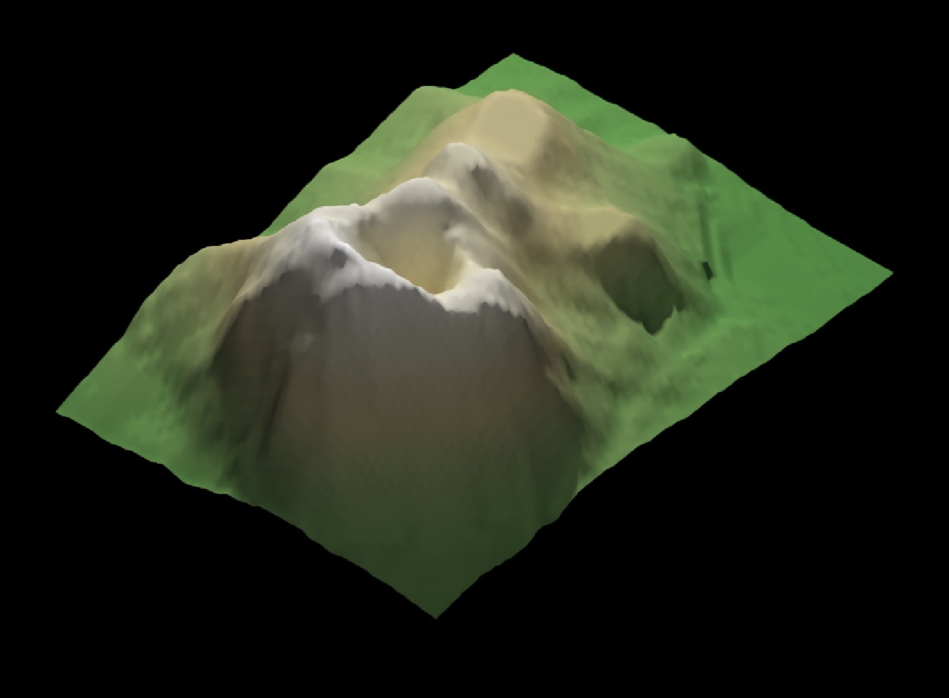
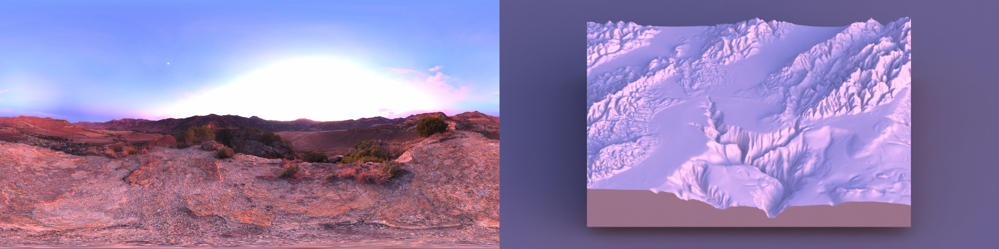
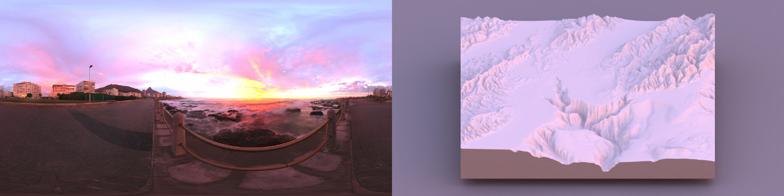
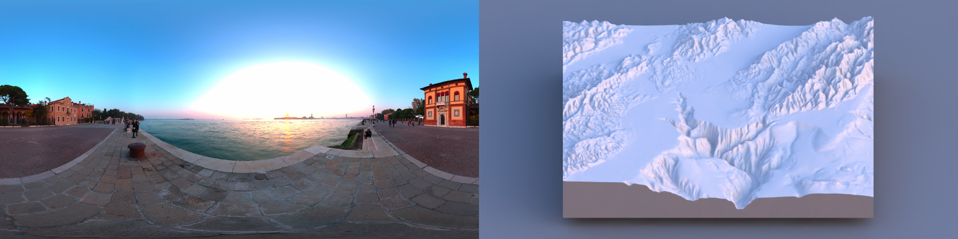
One of the hardest details to get right in 3D data visualization is lighting: since 2D screens don’t offer the benefit of stereoscopic vision, we have to rely on subtle cues like occlusion, relative motion (if animated), and shading to be able to interpret the space as 3D. Nowhere is this more clearly demonstrated than on topographic maps, where shadows can make what is otherwise a largely featureless blob of color transform into a landscape. Add direct light with diffuse shading to a model, and voilà:

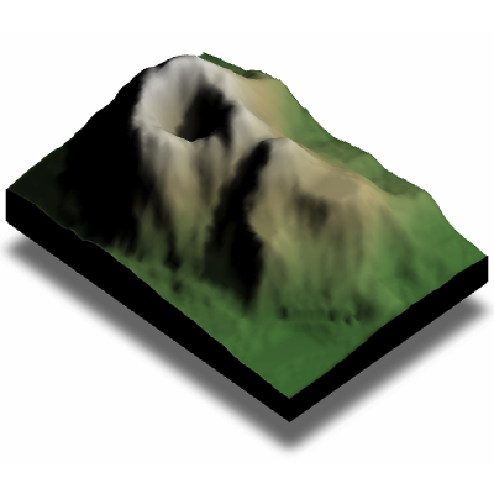
A volcano! Adding basic shading like this allows us to interpret the surface as 3D, even though the medium (your screen) is 2D. This is all perfectly fine and dandy until there’s some detail you want to see in that shaded space. In that case, just using a key light can hide important (key!) information.
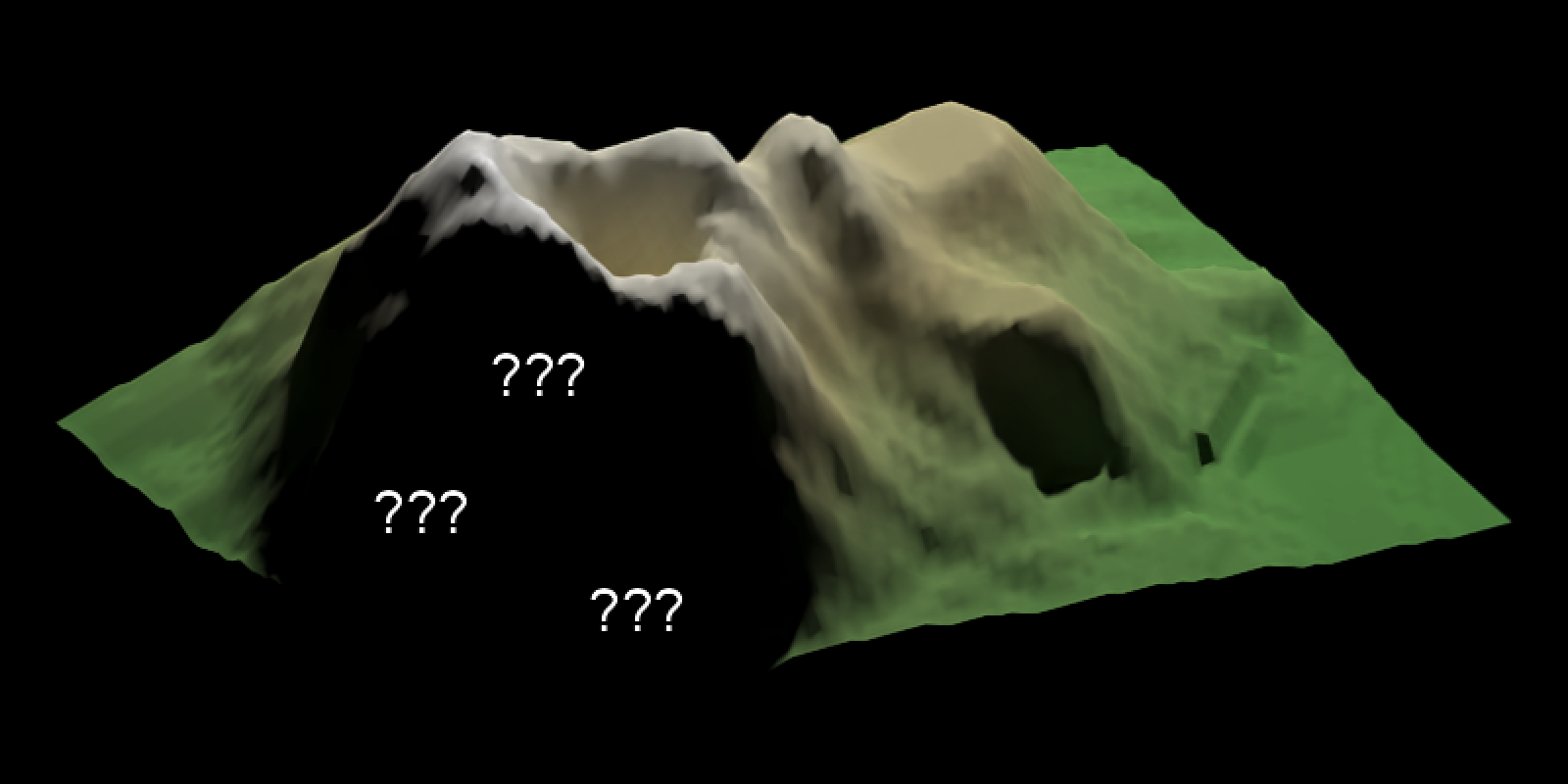
One way to get that information is to use time as a dimension, and animate either the model or the light. For example, if we send a light spinning around the model, we can ensure that everything we want to show is lit at one point, or the viewer can mentally integrate lighting cues over time. A rotating key light (or a slowly orbiting camera) turns shadowing into a transient effect, bringing light to even the darkest of hillsides.
That’s great for exploration and presentations, but it doesn’t help when your deliverable is a single static figure. Thankfully, this issue isn’t unique to dataviz: the problem of how to paint enough light in a scene so the viewer can interpret the space while avoiding overly dark/light areas is also faced by cinematographers and photographers, and we can apply the tools they’ve developed to our domain (3D data visualization).
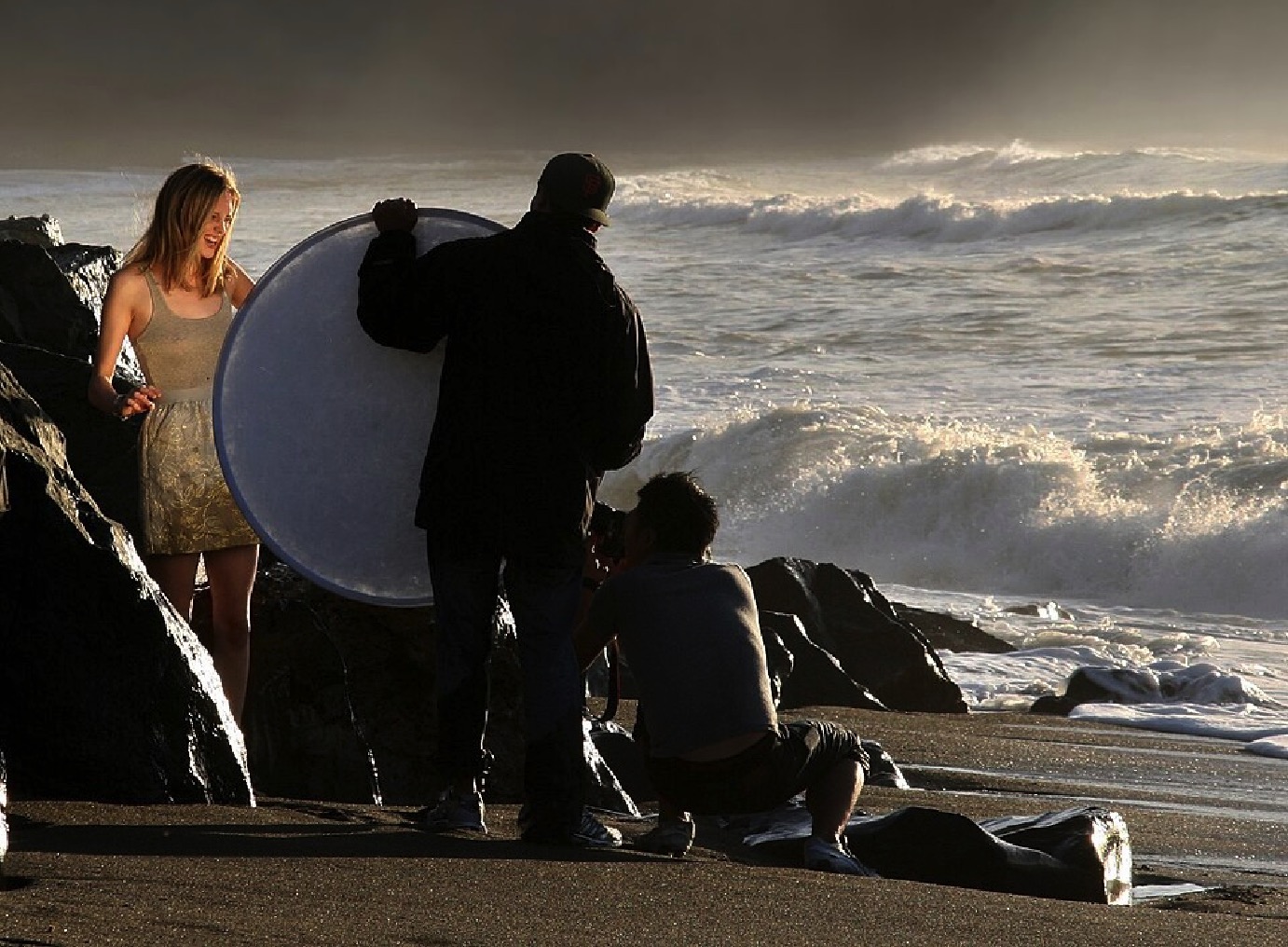
Their solution is to ensure light reaches those regions in deliberate ways, angled in a way that maintains the overall contrast while allowing the contours of shapes to be understood. This is done by adding a fill light: a lower-intensity light coming in from a direction that illuminates the dark region. This can either be a separate light or a large diffuse surface to reflect a strong light source back at the target.
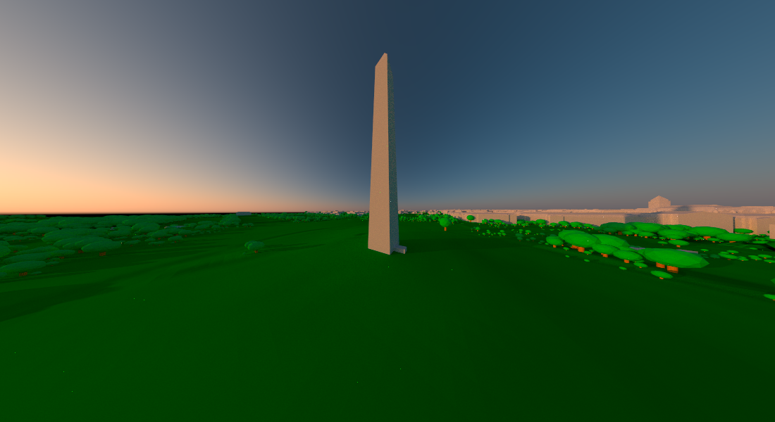
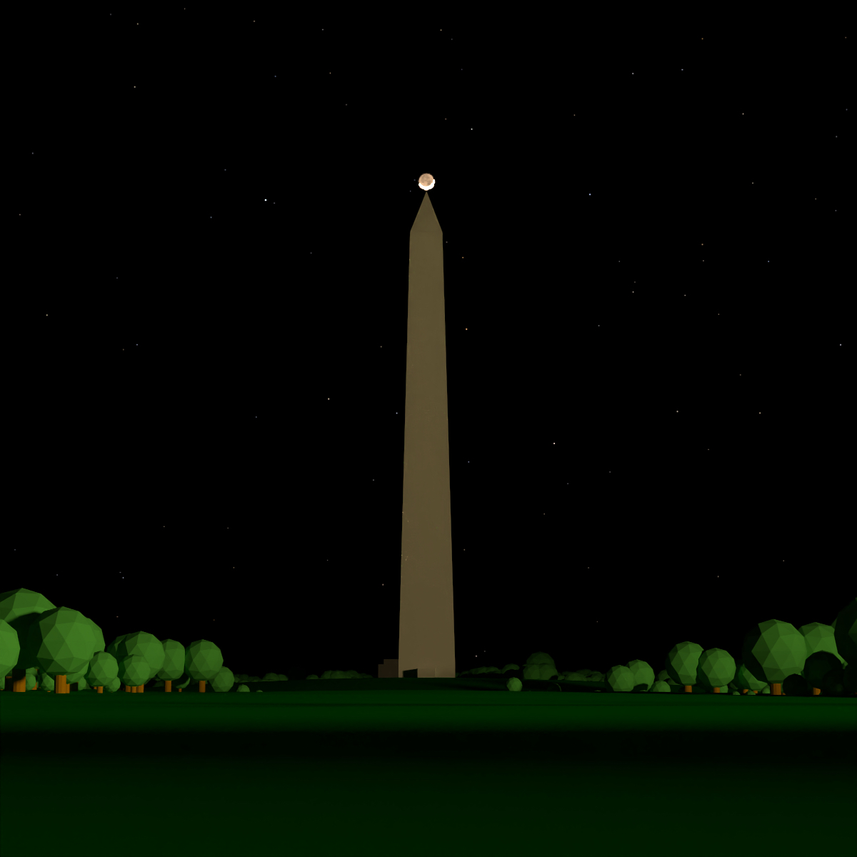
This is okay for simple landscapes, but it becomes problematic as you introduce features which create long shadows. It’s also a pain to arrange the perfect 3D orientation of lights to capture your scene: you have to position three objects in space (camera, fill light, key light) plus determine the right relative intensity of light. It’s a scene-dependent 10D optimization problem. For an example, let’s look at the Washington Monument lit by both a bright key light and a dimmer fill light.
Code
#Set location of Washington Monument
washington_monument_location =  st_point(c(-77.035249, 38.889462))
wm_point = washington_monument_location |>
 st_buffer(0.002) |>
 st_sfc(crs = 4326) |>
 st_transform(st_crs(washington_monument_multipolygonz))

elevation_data = elevatr::get_elev_raster(locations = wm_point, z = 14)

scene_bbox = st_bbox(st_buffer(wm_point,2000))
cropped_data = raster::crop(elevation_data, scene_bbox)

#Use rayshader to convert that raster data to a matrix
dc_elevation_matrix = raster_to_matrix(cropped_data)

#Remove negative elevation data
dc_elevation_matrix[dc_elevation_matrix < 0] = 0

#Plot a 3D map of the national mall
dc_elevation_matrix |>
 constant_shade(color="darkgreen") |>
 add_shadow(lamb_shade(dc_elevation_matrix), 0) |>
 plot_3d(dc_elevation_matrix, zscale=3.7, shadow=FALSE,
         soliddepth=-50, windowsize = 800)
render_multipolygonz(washington_monument_multipolygonz,
                    extent = raster::extent(cropped_data),
                    zscale = 4, color = "grey80",
                    heightmap = dc_elevation_matrix)
render_camera(238,15.5,0.8, fov = 43.4)
render_highquality(lightdirection = c(0,225), lightintensity = c(1500,500), samples=64,
                   width = 800, height=400, lightsize = 200,
                   camera_location =c(72.49, 47.14, -0.53), camera_lookat =  c(-19.75, 8.30, -47.12),
                   lightaltitude=20)
rgl::close3d()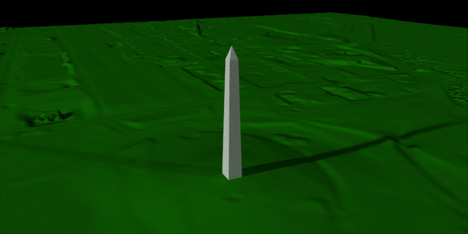
You can see the two lights now create two separate shadows, on top of the shadows from the terrain. With one building on a relatively flat surface it isn’t too bad, but with many buildings or a more complex landscape, all the overlapping shadows can add a lot of visual clutter and noise to an image. To demonstrate, let’s render a fairly normal town center: Figure 6 shows an intersection surrounded by buildings in Monterey, California.
Code
osm_bbox = c(-121.9472, 36.6019,  -121.9179, 36.6385)

opq(osm_bbox) |>
  add_osm_feature("building") |>
  osmdata_sf() ->
osm_data

opq(osm_bbox) |>
  add_osm_feature("highway") |>
  osmdata_sf() ->
osm_road

building_polys = osm_data$osm_polygons
osm_dem = elevatr::get_elev_raster(building_polys, z = 11, clip = "bbox")
e = extent(building_polys)

osm_dem |>
  crop(e) |>
  extent() ->
new_e

osm_dem |>
  crop(e) |>
  raster_to_matrix() ->
osm_mat

osm_mat[osm_mat <= 1] = -2

osm_mat |>
  constant_shade(color = "tan") |>
  plot_3d(osm_mat, water = TRUE, windowsize = c(800, 400), watercolor = "dodgerblue",
          zscale = 10, theta=220, phi=22, zoom=0.45, fov=110,
          background = "pink")

render_buildings(building_polys,  flat_shading  = TRUE,
                 angle = 30 , heightmap = osm_mat,
                 material = "white", roof_material = "white",
                 extent = new_e, roof_height = 3, base_height = 0,
                 zscale=10)
render_camera(fov=5, zoom = 0.04)
render_highquality(lightdirection = c(45,225), lightintensity = c(500,250), lightaltitude = 20,
                   camera_location = c(-1203.09, 756.18, -1433.73),
                   camera_lookat= c(6.43, -1.13, -32.40))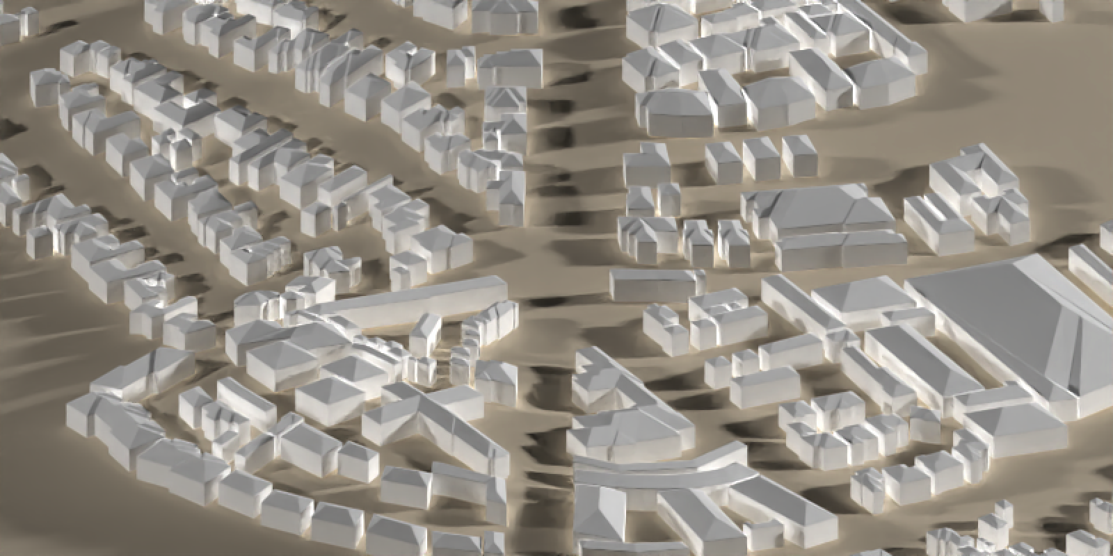
The issue is the sharpness and discreteness of the lights: it’s not aesthetically pleasing to have multiple sharply defined lights, and the marginal additional context the fill light provides is strongly counteracted by the visual mess it creates. Photographers face the same issue when capturing people in sunlight: direct sunlight creates unflattering and distracting sharp shadows across the face. What we need is some sort of gradual variation in light across the sky that provides a soft bright light but without sharp edges, something that provides the same overall directional information without the sharp lines. Thankfully, photographers have long figured out the solution to this, and it’s called… a sunset.
The golden hour… for dataviz?
There are two properties of sunsets that make for great photos, and thus (for our purposes) great 3D renderings. First, the atmosphere greatly attenuates direct sunlight close to sunset, making the difference between the direct and indirect lit areas on the subject much less stark, often described as the lighting ratio in cinematography. This lowers the contrast, softening those sharp lines. Cinematographers often target lighting ratios between 3:1 and 2:1 (in stops, which scale as \(2^s\); 8:1 to 4:1 in linear terms) for illuminating faces1. Second, the thicker atmosphere at lower solar elevation angles scatters more short-wavelength light from the sun, producing warmer tones at sunrise. This dependence on solar elevation leads us to a fairly common definition of “golden hour:” when the sun is \(\approx -6^\circ\) to \(\approx 6^\circ\) from the horizon.
Figure 7 shows a chart of the CIE xy 1931 chromaticity diagram including the Planckian Locus. The Planckian locus is the path that a black body color will take through the diagram as the temperature changes. The hue of sunlight shifts from the right side of the black line to the left as the sun rises, and the time it spends in the yellow/red region is our “golden hour” lighting.
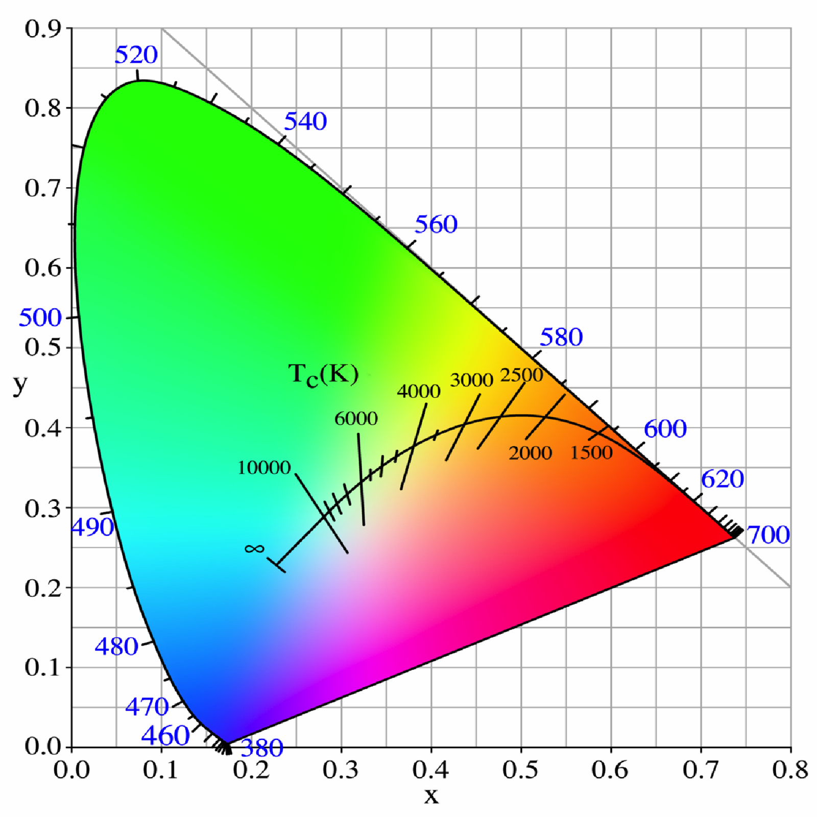
This color change results in dramatic color gradation across the sky (from orange hues near the sun to blues opposing it, which are still scattered blue indirect light) that naturally contours objects by color, versus providing that spatial contouring via shadow/light. Cinematographers use this technique all the time: cool/warm lights are often used as proxies for dark/light areas, allowing viewers to pick up on small changes in actors’ faces (for emotions, and whatnot) that might have been lost if half the actor’s face had been bathed in darkness.

HDR Environment Maps
There’s one easy way to add a sunset to a scene when pathtracing: an environment image. This is basically a \(360^\circ\) HDR image of the real world that you use to light your scene. And thankfully, there’s a whole community of photographers who have provided these for free online, which you can find at Polyhaven. Environment lights are great because you get complex, natural lighting without micromanaging individual lights. Some of my favorites from Polyhaven are the following (click on a tab to stop cycling):
Code
render_monterey = function(env_light = "kiara_1_dawn_2k.hdr", iso=100, samples=32,
                           ground_color ="grey20", shadow = TRUE, zoom = 0.45) {
  montereybay |>
    constant_shade(color="grey40") |>
    plot_3d(montereybay, windowsize = c(800,400), zscale=50, shadow = shadow)
  render_camera(zoom=zoom,theta=-90,phi=30)
  rayval = render_highquality(environment_light = env_light, iso = iso, samples = samples,
                     light=FALSE, water_ior = 1.2,
                     ground_material = diffuse(color=ground_color), preview=FALSE, plot = FALSE)
  rgl::close3d()
  return(rayval)
}
Note that the sunset still gives a relatively bright highlight on the mountaintops, but the shadows otherwise are fairly soft throughout the terrain. And while the highlights are significantly brighter than the shaded regions, the bright and dark regions aren’t too different: we have just the right amount of contrast.
The obvious follow-up is: what happens when we choose a non-sunset? Here are a few examples of other environment lights from Polyhaven, taken either midday or indoors, with some more structured discrete lighting. Let’s see what those look like:
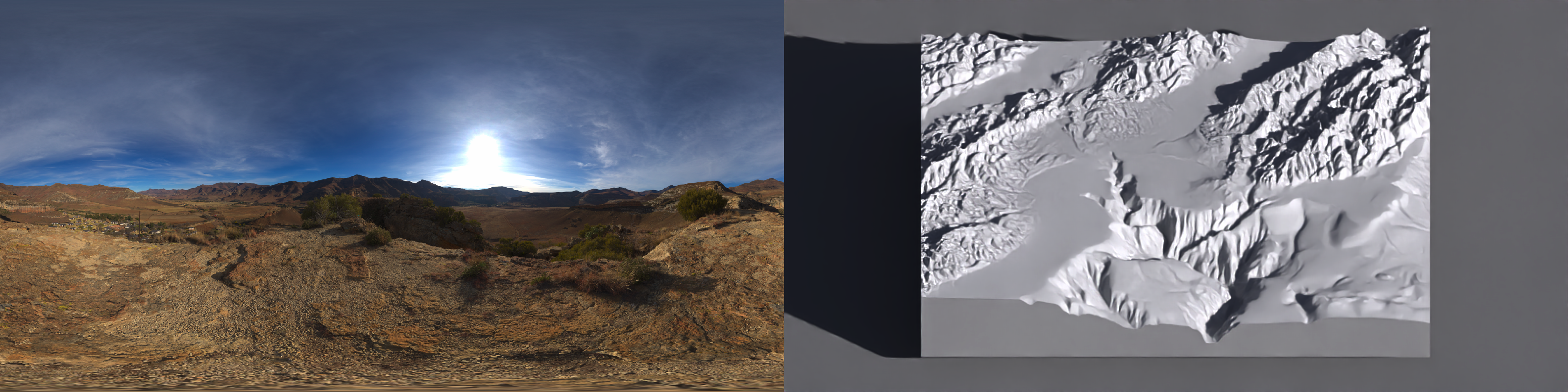
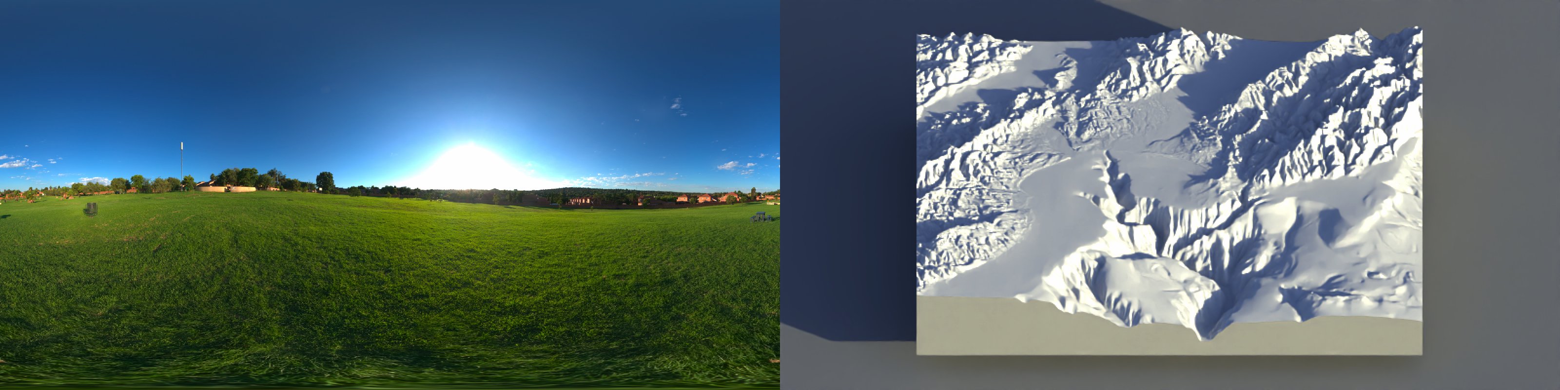
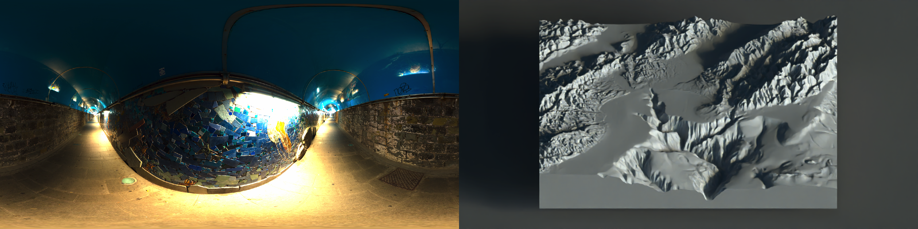
The primary problem we face here is the lack of balance between the shading from the ambient sky lighting and the direct light from the sun. Note the sharp shadow edges interspersed throughout the landscape and the dark shadows: one strong light tends to overwhelm everything around it. There’s too much contrast between the dark areas and the light areas: the light from the key light (here, the sun) dominates the image.
The hillshading surface ambiguity
And this isn’t just an aesthetic preference: direct lighting by itself doesn’t provide enough information to unambiguously reconstruct the 3D surface from a 2D projection. It’s a perceptual shortcoming of the hillshading method. Direct light (like from the sun) does allow you to judge the aspect (directionality) of a slope, but it suffers from one major flaw: it’s ambiguous whether you’re looking at a hill or a valley, unless you have long shadows (which we have seen above can cause other issues).
Mathematically, Lambertian lighting darkens the surface via the dot product between the light and the surface normal \(I_{\text{dir}}(x,y) \propto \max\bigl(0,\ \mathbf{v}_{\text{light}}\cdot \mathbf{v}_{\text{normal}}(x,y)\bigr)\)
For a height field (z = h(x,y)), a (unit) surface normal can be written as
\[ \frac{1}{\sqrt{h_x^2+h_y^2+1}} \begin{bmatrix} -h_x\\ -h_y\\ 1 \end{bmatrix} \]
where
\[ h_x=\frac{\partial h}{\partial x},\ \ h_y=\frac{\partial h}{\partial y}. \]
The hill/valley ambiguity is a sign ambiguity: if you invert the terrain (\(h \mapsto -h\)), then (\((h_x,h_y)\mapsto(-h_x,-h_y)\)), the normal becomes
\[ \frac{1}{\sqrt{h_x^2+h_y^2+1}} \begin{bmatrix} +h_x\\ +h_y\\ 1 \end{bmatrix}. \]
Now decompose the light direction into horizontal and vertical components (\(\mathbf{v}_{\text{light}} = [\ell_x,\ \ell_y,\ \ell_z,]^T\)) with (\(|\mathbf{v}_{\text{light}}|=1\)). The Lambertian dot product is
\[ \mathbf{v}_{\text{light}}\cdot \mathbf{v}_{\text{normal}} = \frac{-\ell_x h_x - \ell_y h_y + \ell_z}{\sqrt{h_x^2+h_y^2+1}}, \qquad \mathbf{v}_{\text{light}}\cdot \mathbf{v}_{\text{normal}}' = \frac{+\ell_x h_x + \ell_y h_y + \ell_z}{\sqrt{h_x^2+h_y^2+1}}. \]
If you also flip the horizontal light direction (equivalently rotate azimuth by \(180^\circ\)), (\(\mathbf{v}_{\text{light}}'=[-\ell_x,\ -\ell_y,\ \ell_z]^T\)), then
\[ \mathbf{v}_{\text{light}}'\cdot \mathbf{v}_{\text{normal}}' = \frac{-\ell_x h_x - \ell_y h_y + \ell_z}{\sqrt{h_x^2+h_y^2+1}} = \mathbf{v}_{\text{light}}\cdot \mathbf{v}_{\text{normal}} \]
So the directed shading field is identical under the paired transformation
\[ (h, \mathbf{v}_{\text{light}})\mapsto (-h,\ [ -\ell_x,\ -\ell_y,\ \ell_z]^T) \]
i.e., “hill with light from azimuth (\(\phi\))” produces the same Lambertian shading as “valley with light from azimuth (\(\phi+\pi\))”).
We can demonstrate this effect by visualizing the same terrain, first visualized normally and then visualized inverted with the sun flipped around:
Code
montereybay |>
  lamb_shade(zscale=30, sunangle = 315) |>
  plot_3d(montereybay, zscale=30, windowsize=600, zoom=0.9)

output1 = render_movie(frames = 120, theta = rep(55,120), type="custom",
             phi = tweenr::tween_t(c(90,45,90),n=120,ease="cubic-in-out")[[1]],
             zoom=rep(0.9,120),filename="innie.mp4")
rgl::close3d()

-montereybay |>
  lamb_shade(zscale=30, sunangle = 315+180) |>
  plot_3d(-montereybay, zscale=30, windowsize=600)

output2 = render_movie(frames = 120, theta = rep(55,120), type="custom",
             phi = tweenr::tween_t(c(90,45,90),n=120,ease="cubic-in-out")[[1]],
             zoom=rep(0.9,120),filename="outie.mp4")
rgl::close3d()
system("ffmpeg -y -i innie.mp4 -i outie.mp4 -filter_complex hstack -pix_fmt yuv420p ../videos/2026/inner_outie.mp4")
Figure 9 shows that when the camera is directly overhead, the two hillshades are identical. The traditional solution cartographers developed for this problem (and have stuck with for several centuries) is to stick with one convention for the direction of light, for all maps, until the heat death of the universe: Northwest, or \(315^\circ\). With the idea being that if every terrain map is always lit from the same direction, you’ll never encounter this ambiguity, because you have been subliminally trained your entire life to see light coming from the northwest.
Or, in other words, a cartel of cartographers formed an illumination illuminati to plot an influence campaign so you would understand their plots.
This convention is a little odd, however, because you only encounter light coming from the northwest near the poles. Greater than \(55.8^\circ\) latitude, to be exact: in effect, all terrain maps are pretending to be Norwegian.
In a post on this very issue, the cartographer Tom Patterson discussed an interesting hypothesis on why northwest ended up becoming the standard in hillshading:
“Because most people are right handed, when we write or draw we tend to place desk lighting above and to the left so as not to cast shadows over our work. Moreover, our work generally progresses from upper left to lower right, minimizing the possibility for smearing. […] When depicting shaded relief and other 3D phenomena on a flat sheet of paper, we naturally take a cue from the lighting within our work place environment and apply shadows to the lower right sides of slopes. Centuries of depicting topography in this manner has ingrained this cartographic convention.”
Adding ambient shading solves this ambiguity by breaking the symmetry: it models how much of the sky is visible at each point, so valleys are darkened while ridges are not. By layering an ambient layer with the direct lighting layer, it becomes clear what is a valley and what is a ridge. But these two terms need to be fairly balanced: if the key light term dominates, it is harder for the ambient term to break the ambiguity.
Code
montereybay |>
  constant_shade() |>
  add_shadow(lamb_shade(montereybay, zscale=100),0) |>
  plot_map()

montereybay |>
  constant_shade() |>
  add_shadow(ambient_shade(montereybay, zscale=5),0) |>
  plot_map()

montereybay |>
  constant_shade() |>
  add_shadow(ambient_shade(montereybay,zscale=5),max_darken = 0) |>
  add_shadow(lamb_shade(montereybay,zscale=100),max_darken = 0) |>
  plot_map()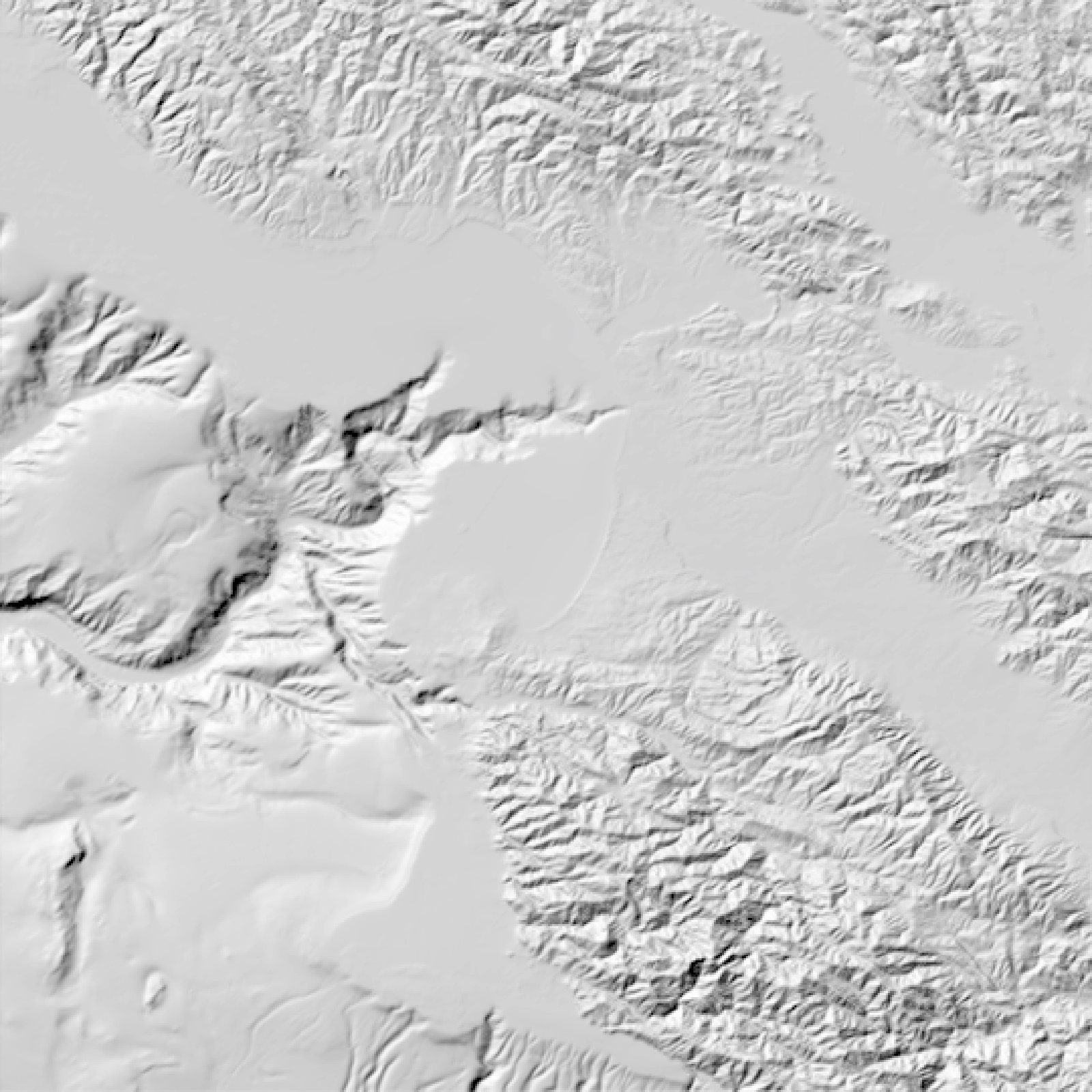
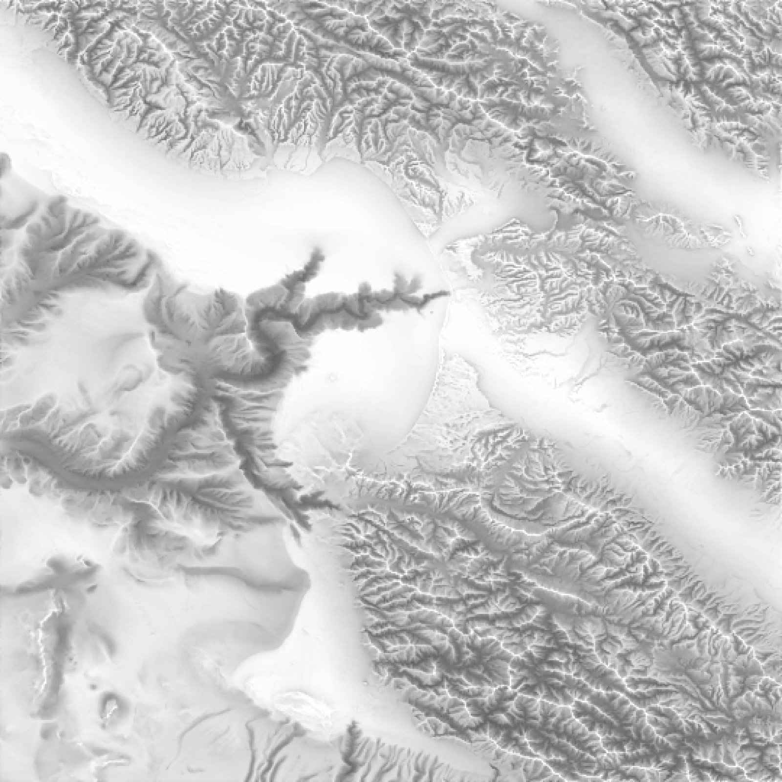
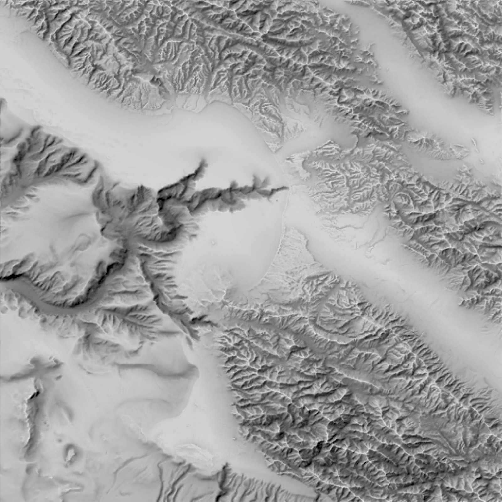
Sunset contrast, hues, and lighting ratios
This solution is great for 2D hillshades, but it also gives us a good rule of thumb to help make static 2D projections of 3D visualizations more interpretable: When your lighting results in these two terms being around the same intensity, you’re likely in a good place visually. Sunsets and sunrises offer much more balanced amounts of direct and indirect light than the mid-day sun, so surfaces retain clear directional shading without plunging half the scene into near-black shadow: you get shape cues and visible detail in valleys, crevices, and between structures, with far less harsh edge contrast. In fact, if by some chance we had an accurate model of the indirect and direct lighting from the atmosphere (spoiler alert!), we could compare the hue and brightness from opposite sides of the atmosphere and see how the lighting ratio and color change with solar elevation. We might get something like this:
Code
hue_diff_oklab_linear_srgb = function(rgb1, rgb2, sat_eps = 0.02) {
stopifnot(length(rgb1) == 3, length(rgb2) == 3)
if (!requireNamespace("farver", quietly = TRUE)) {
stop("Install farver: install.packages('farver')")
}
rgb = rbind(as.numeric(rgb1), as.numeric(rgb2))
rgb = pmax(rgb, 0)
M = matrix(
c(0.4124, 0.3576, 0.1805,
0.2126, 0.7152, 0.0722,
0.0193, 0.1192, 0.9505),
nrow = 3, byrow = TRUE
)
xyz = rgb %*% t(M)
oklab = farver::convert_colour(
xyz, from = "xyz", to = "oklab",
white_from = "D65", white_to = "D65"
)
L = oklab[, 1]
a = oklab[, 2]
b = oklab[, 3]
C = sqrt(a^2 + b^2)
sat = C / pmax(L, 1e-12)
if (any(sat < sat_eps) || any(!is.finite(sat))) return(NA_real_)
h = atan2(b, a) * (180 / pi)
abs(((h[2] - h[1] + 180) %% 360) - 180)
}
ratio_to_stops = function(ratio) log(ratio, base = 2)
luma_from_rgb = function(rgb) {
0.2126 * rgb[, 1] + 0.7152 * rgb[, 2] + 0.0722 * rgb[, 3]
}
img_stats = function(rgba) {
R = rgba[, , 1]
G = rgba[, , 2]
B = rgba[, , 3]
rgb = cbind(R, G, B)
Y = luma_from_rgb(rgb)
list(
luma = stats::median(Y, na.rm = TRUE),
rgb = c(mean(R, na.rm = TRUE), mean(G, na.rm = TRUE), mean(B, na.rm = TRUE))
)
}
calculate_values = function(elev_angle = 10, dimval = 1500, dist = 10,
ortho_size = 0.05, samples = 256,
save_dir = ".", save_renders = TRUE) {
skyfile = tempfile(fileext = ".exr")
skymodelr::generate_sky(
azimuth = 180,
resolution = dimval,
elevation = elev_angle,
number_cores = 8,
hosek = FALSE,
render_mode = "all",
filename = skyfile
)
common_args = list(
sphere(radius = 0.5, material = diffuse()),
samples = samples, denoise = FALSE, bloom = FALSE, min_adaptive_size = 1,
fov = 0, # orthographic
ortho_dimensions = c(ortho_size, ortho_size), # small "metering window"
preview = FALSE,
lookat = c(0, 0, 0),
environment_light = skyfile,
transparent_background = TRUE
)
img_key = do.call(render_scene, c(common_args, list(lookfrom = c(0, 0, -dist))))
img_fill = do.call(render_scene, c(common_args, list(lookfrom = c(0, 0, dist))))
s_key = img_stats(img_key)
s_fill = img_stats(img_fill)
ratio = s_key$luma / pmax(s_fill$luma, 1e-6)
stops = ratio_to_stops(ratio)
hue_diff = hue_diff_oklab_linear_srgb(s_fill$rgb, s_key$rgb, sat_eps = 0.02)
if (isTRUE(save_renders)) {
fn_key = file.path(save_dir, sprintf("patch_key_elev_%+03d.png",
as.integer(round(elev_angle))))
fn_fill = file.path(save_dir, sprintf("patch_fill_elev_%+03d.png",
as.integer(round(elev_angle))))
rayimage::ray_write_image(img_key, fn_key)
rayimage::ray_write_image(img_fill, fn_fill)
}
data.frame(
key_level = s_key$luma,
fill_level = s_fill$luma,
ratio = ratio,
stops = stops,
hue_diff = hue_diff,
elevation = elev_angle
)
}
elevation_angles = seq(0, 20, by = 1)
lighting_ratio = lapply(elevation_angles, \(a) calculate_values(a, dimval = 5000))
lighting_ratio_df = do.call(rbind, lighting_ratio)- 1
- Compute hue separation in OKLab from two linear-sRGB RGB triplets, with a saturation gate to avoid unstable hue near gray.
- 2
- Clamp negative channels before color transforms (defensive against numerical noise).
- 3
- Convert linear sRGB to XYZ (D65) with a standard matrix.
- 4
-
Convert XYZ to OKLab with
farver. - 5
-
Compute chroma and relative saturation (
C/L); returnNAif either side is too desaturated. - 6
- Compute the shortest-path hue angle difference (degrees).
- 7
-
Convert a linear key/fill ratio to stops using
log2(). - 8
- Compute linear luminance from linear RGB (no transfer curve).
- 9
- Summarize a rendered RGBA patch.
- 10
- Extract RGB samples and compute per-pixel luminance.
- 11
- Use median luminance (robust brightness) and mean RGB (representative color) over the patch.
- 12
- Full measurement for one solar elevation with a small orthographic “metering window”.
- 13
- Allocate a temporary EXR filename for the sky environment map.
- 14
- Generate the sky (Prague) for the given solar elevation.
- 15
- Centralize common render arguments to keep key/fill renders identical except for viewpoint.
- 16
-
Use orthographic projection (
fov = 0) so the “patch” is a literal fixed-size window in scene units. - 17
-
Set
ortho_dimensionsto a small size (e.g.0.05 x 0.05) so the entire render is the sampled region. - 18
-
Render the key-side patch from
lookfrom = (0,0,-dist)toward the origin. - 19
-
Render the fill-side patch from the opposite viewpoint
lookfrom = (0,0,+dist)(180 degrees opposed). - 20
- Compute per-side brightness and mean color from the full patch image.
- 21
- Compute key/fill ratio and convert to stops.
- 22
- Compute hue difference between the two patch-average colors in OKLab.
- 23
- Optionally write the two sampled patch renders to disk for inspection.
- 24
- Return a tidy row with brightness, ratio/stops, hue difference, and elevation.
- 25
- Sweep over elevations and row-bind results into a single data frame.
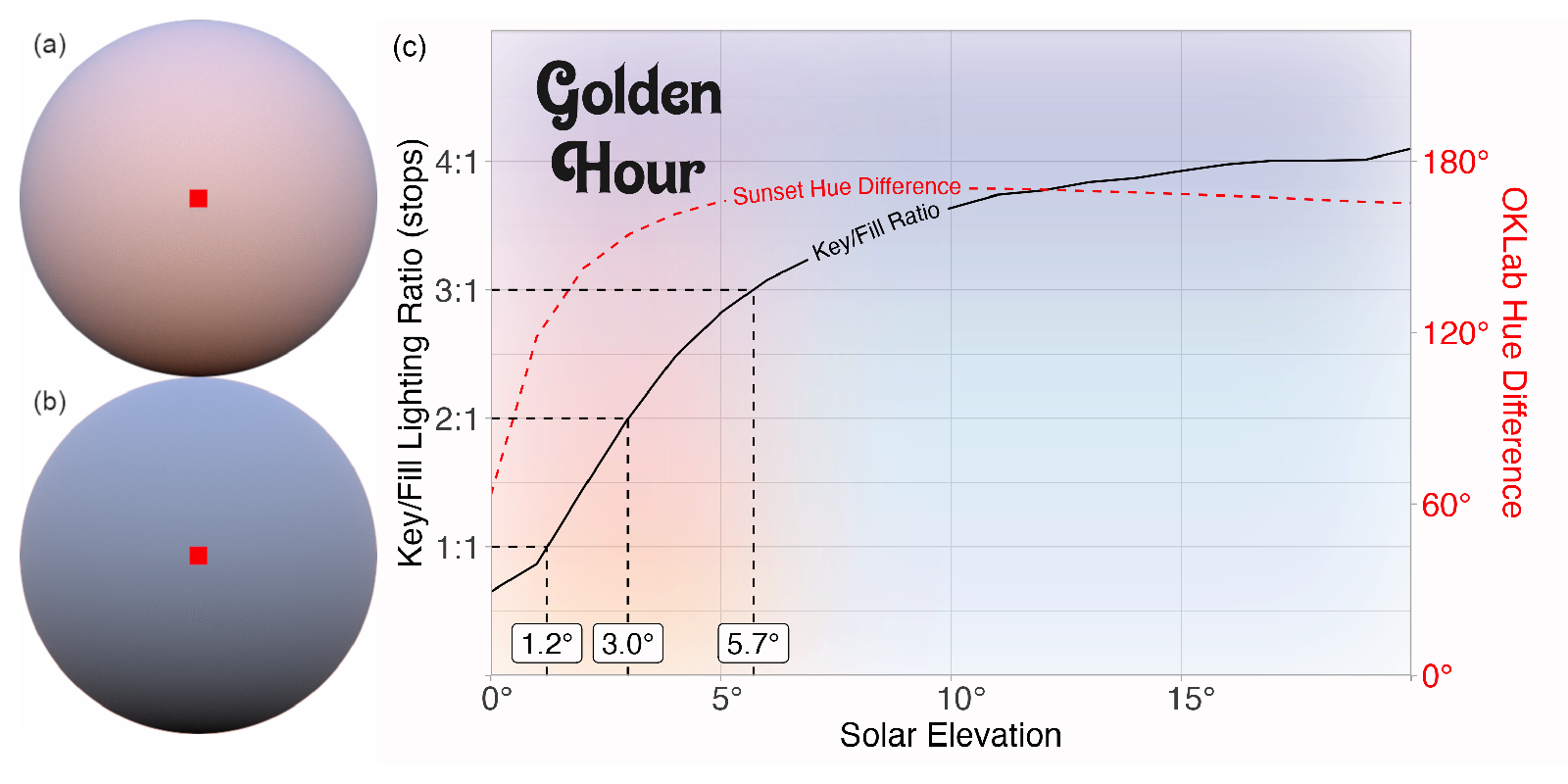
Figure 13 shows that the lighting ratio reaches the cinematography sweet spot of 3:1 right around \(6^\circ\), which also happens to be the commonly stated range for when the photographic golden hour begins! We also see that while the lighting ratio decreases, the color (hue) shift stays fairly high across shapes until very low solar elevations. The difference between the red curve and the black is what makes the golden hour so magical: as the contrast between the fill and the key light decreases, the difference in hues between the two sides becomes more apparent. Sunset is thus the period of time when objects are primarily contoured in color, rather than in brightness.
The problem with HDR images as environment lights
So HDR environment images of sunsets provide an easy way to get natural, soft lighting that’s easy to interpret. However, there are downsides to environment lights. Because the image is fixed, there’s not much you can do to customize the light. You can rotate it, but the overall color and light distribution with respect to the horizon can’t be changed. Also, with that beautiful real-world lighting often come pesky real-world people and objects: it might be confusing why someone is behind your scene, staring back at your viewer.
This isn’t an issue if you’re always looking down on the map from above, but for oblique views this is a huge drawback. Good data visualization designers know that every element in a visualization should serve a purpose; everything in a dataviz that doesn’t in some way contribute to a reader’s understanding lowers the visualization’s signal-to-noise ratio. And that’s bad.
It would be nice to have a clean, customizable environment map that gives us that pristine golden-hour light without any real-world interlopers. Is this a realistic goal–or is it just a pie in the sky dream?
Generating a synthetic sky
The dumber the joke, the more research it deserves
Thankfully, graphics researchers have developed two atmospheric models within the last 15 years that do just that. These models take atmospheric and positional inputs (such as viewer altitude, visibility, atmospheric turbidity, and sun position) and return radiance values for various angles, altitudes, and light wavelengths. We can calculate what the sky would look like for a given set of inputs by sampling on a sphere and then writing that to an environmental light. I’ve written an R package, skymodelr, that does all of that (and more): it generates HDR environment maps given a desired set of atmospheric inputs.
The most basic function available is generate_sky(): you specify a sun position in the sky (azimuth and angle around the sphere), and it generates a sky model. We can then pass this environmental light to our scene. Note that since we’re using realistic lighting, we need to adjust the exposure for proper display on the web.
library(skymodelr)

generate_sky(resolution = 800,
             azimuth = 180,
             elevation = 20,
             hosek = FALSE,
             filename="demo_sky.exr") |>
  render_exposure(-6) |>
  plot_image()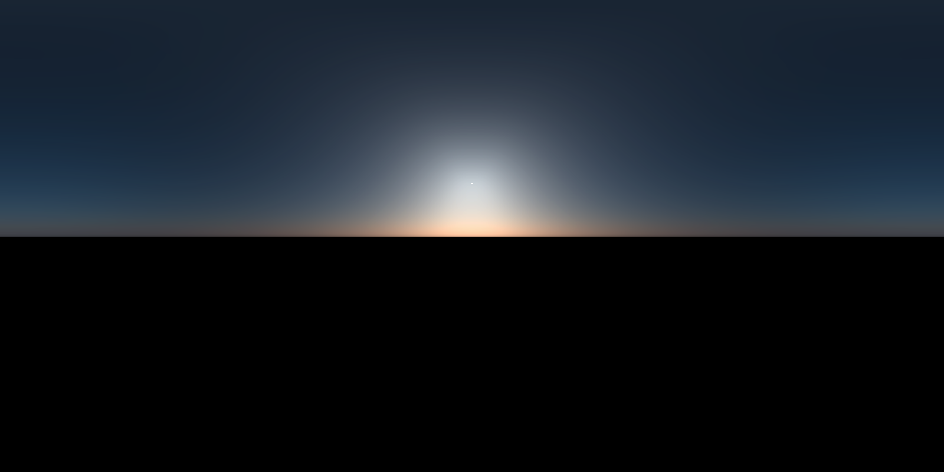
library(skymodelr)

generate_sky(resolution = 800,
             azimuth = 180,
             elevation = 20,
             hosek = FALSE,
             filename="demo_sky.exr") |>
  # No exposure adjustment
  plot_image()
From radiance to RGB
Honestly, you can skip this section and proceed onwards unless you’re interested in the nuts and bolts of how the package turns spectral radiance measurements into colors on your screen. I won’t be offended. Truly.
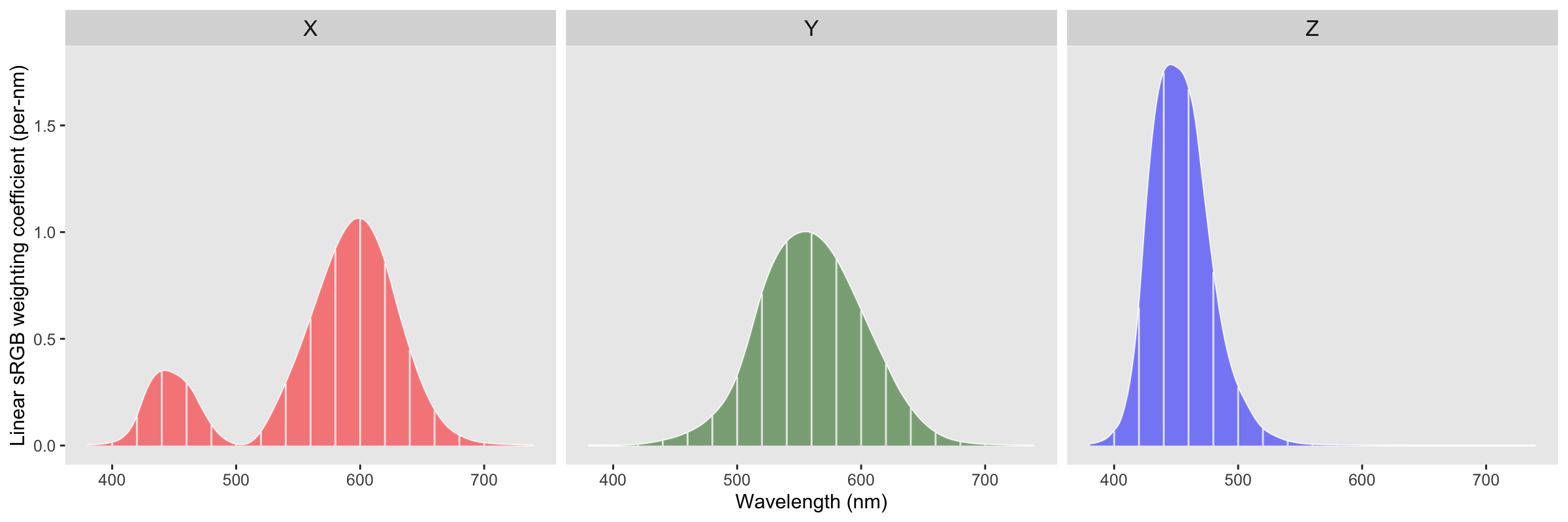
The atmospheric model returns spectral radiance values at a fixed set of wavelengths (in this implementation, the Prague model is evaluated on an 18-band grid from 360 to 700 nm in 20 nm steps). To turn those spectral samples into an RGB image, we approximate the continuous spectral-to-color integral: each wavelength contributes to perceived color in proportion to the CIE 1931 2-degree color matching functions (\(\bar{x}\), \(\bar{y}\), \(\bar{z}\)), which map monochromatic light into CIE XYZ tristimulus space (basically, a vector space designed to match our perception of color).
We then map into the linear sRGB space displayed on our monitors with a 3 x 3 linear transform (assuming a D65 white point and the standard sRGB primaries). Written explicitly,
\[ \begin{bmatrix} R \\ G \\ B \end{bmatrix} = \begin{bmatrix} \phantom{-}3.2406 & -1.5372 & -0.4986 \\ -0.9689 & \phantom{-}1.8758 & \phantom{-}0.0415 \\ \phantom{-}0.0557 & -0.2040 & \phantom{-}1.0570 \end{bmatrix} \begin{bmatrix} X \\ Y \\ Z \end{bmatrix} \]
Multiplying this matrix with our XYZ curve gives us our spectrum-to-RGB weights:
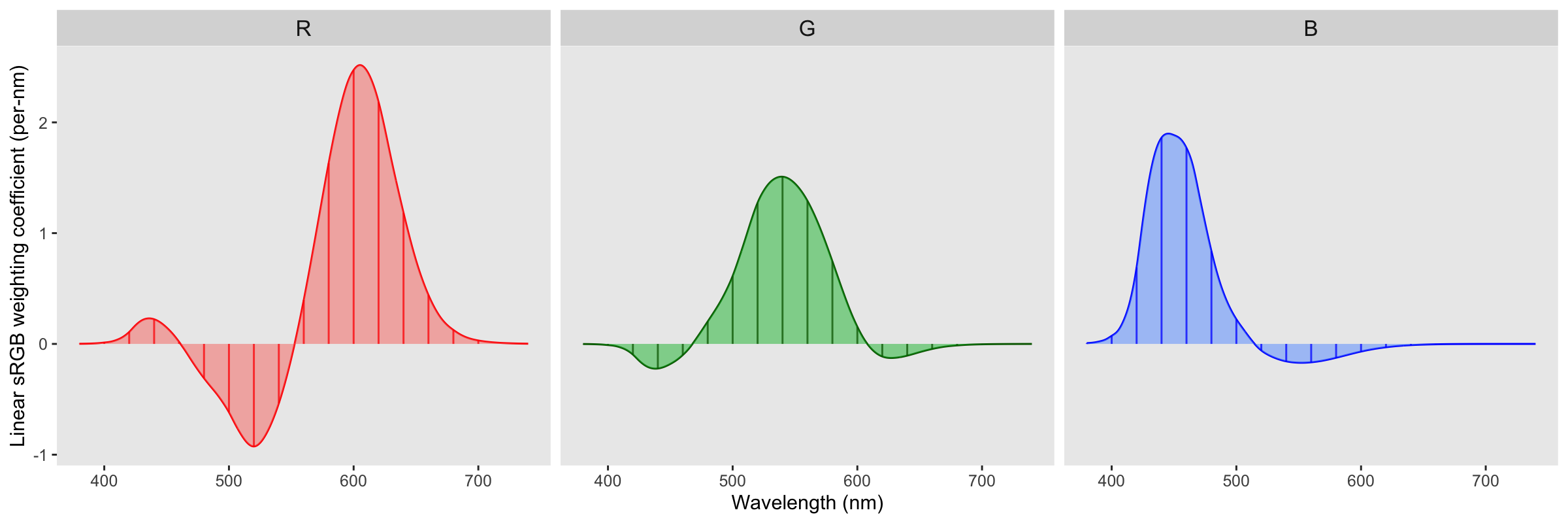

The triangle region represents the gamut of the sRGB colorspace: you can see there are a lot of colors that we can perceive (the area outside the triangle) that sRGB can’t represent.
From here, each pixel direction in the sky dome yields a spectrum \(L(\lambda_i)\), which we reduce to an RGB triplet via the weighted sum above. Interpreting the result as radiance, we store it in a latitude-longitude environment map. During rendering, the environment map acts as a distant light source: a shading point samples directions on the hemisphere, queries the environment radiance for those directions, and accumulates the resulting light.
Bringing OpenEXR to R
Because the Prague model strives for accuracy and returns realistic radiance values for each wavelength, after we run this mathematical machinery we get extremely high brightness values: even the scattered atmospheric light will blow out a low-dynamic range image format like a PNG (which can only represent 8 stops of dynamic range). If we save the image in a format that preserves the full dynamic range, we can adjust the exposure in a post-processing step. Basically, we need to save our images in the rendering equivalent of a photographic RAW image: the OpenEXR format, which preserves the full dynamic range of images. It does this by saving images in arrays of half (16-bit floats) or optionally full floats. Saving images in EXR in R is possible because I spent a good portion of 2025 getting the OpenEXR infrastructure (libopenexr/libimath/libdeflate) onto the CRAN to bring full EXR support to R. This is all wrapped up in the libopenexr package, which provides the write_exr() and read_exr() functions, as well as static libraries to link into compiled code. EXR images bring a much wider dynamic range than standard web formats, allowing you to losslessly capture and process realistic, high-dynamic range content. So any scene rendered with atmospheric lighting saved in the EXR format will have all the precision preserved and allow for post-render exposure control.
| Format | Dynamic range (stops) | Approx. ratio (max / min) |
|---|---|---|
| JPEG 8-bit | 8 | 28 = 256 : 1 |
| PNG 8-bit | 8 | 28 = 256 : 1 |
| PNG 16-bit | 16 | 216 = 65,536 : 1 |
| Outdoor scene | ≈25–35 (scene-dependent) | 230 ≈ 1 billion : 1 |
| OpenEXR Half | ≈ 30 | 230 (40 incl. subnormals) ≈ 1 billion : 1 |
| OpenEXR Float | ≈ 255 | 2255 normal (277 incl. subnormals) ≈ 1076 : 1 (effectively unlimited) |
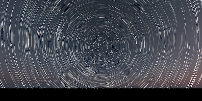
skymodelr saves images with full float precision, which is important if you’d want to do something like, let’s say, add realistic star field rendering to the package. Half has plenty of theoretical headroom, but its shadow precision behaves like a low-bit-depth capture once you expose for the highlights; stars are extremely faint and can end up below the effective noise/quantization floor. This is a problem if you want to do something fun like render realistic star trails from a long exposure.
In the real world, cranking up ISO to increase the contrast of an underexposed image also boosts noise, as you’re amplifying a signal with a low signal-to-noise ratio. In our artificially rendered world we don’t have to worry about that: we have an idealized camera with no noisy electronics measuring our image, so we can freely scale our image into whatever range we need. In fact, we can render all of our images at whatever ISO we want and rescale them afterwards with rayimage::render_exposure(). I use both methods, because adjusting exposure in stops (which scale as \(2^s\)) is good for when you’re way off, but sometimes you just need a slight linear tweak to capture a highlight, which you can do by adjusting the ISO.2
render_monterey("demo_sky.exr", iso = 5) |>
  plot_image()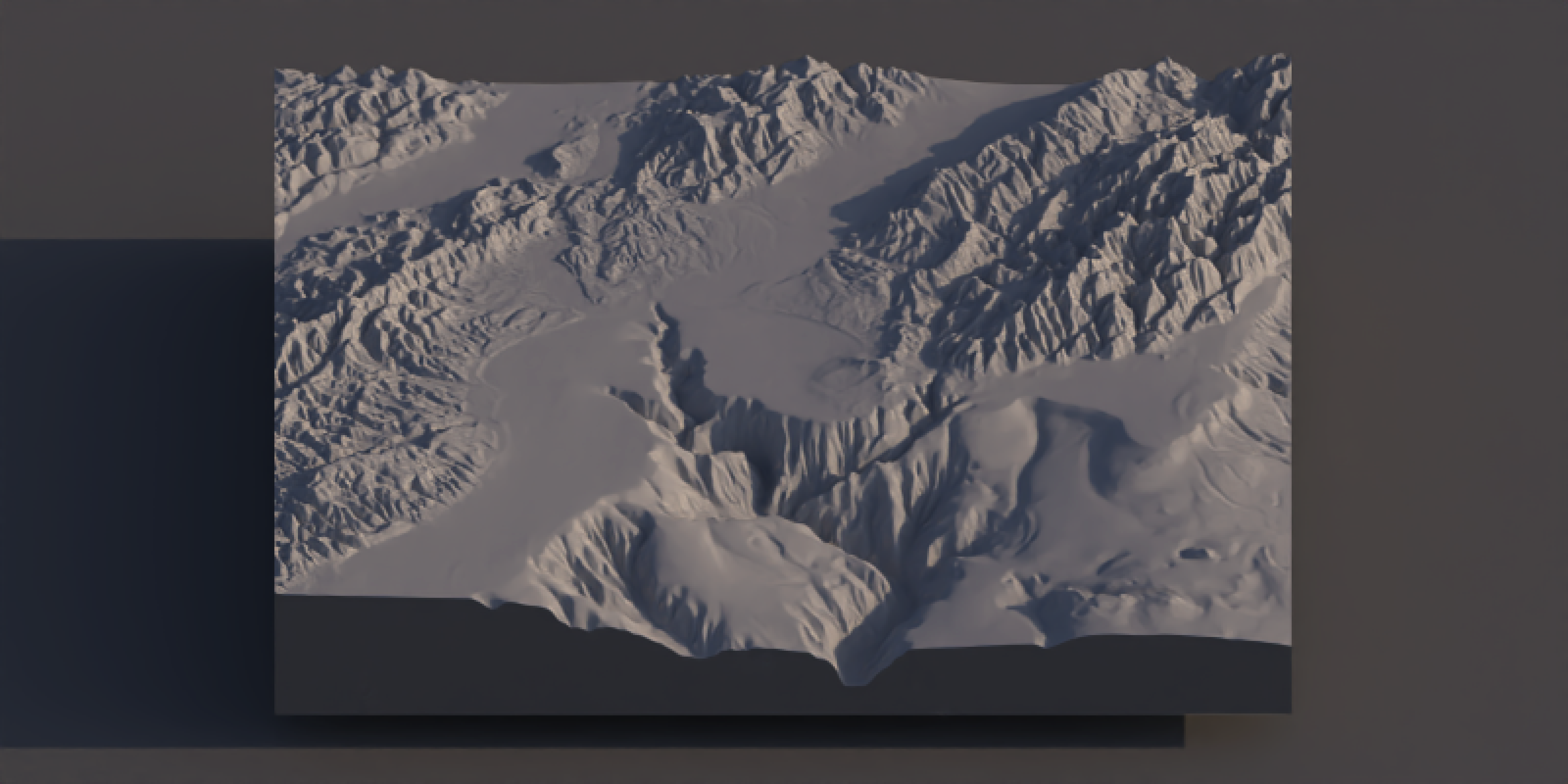
render_monterey("demo_sky.exr", iso = 10) |>
plot_image() 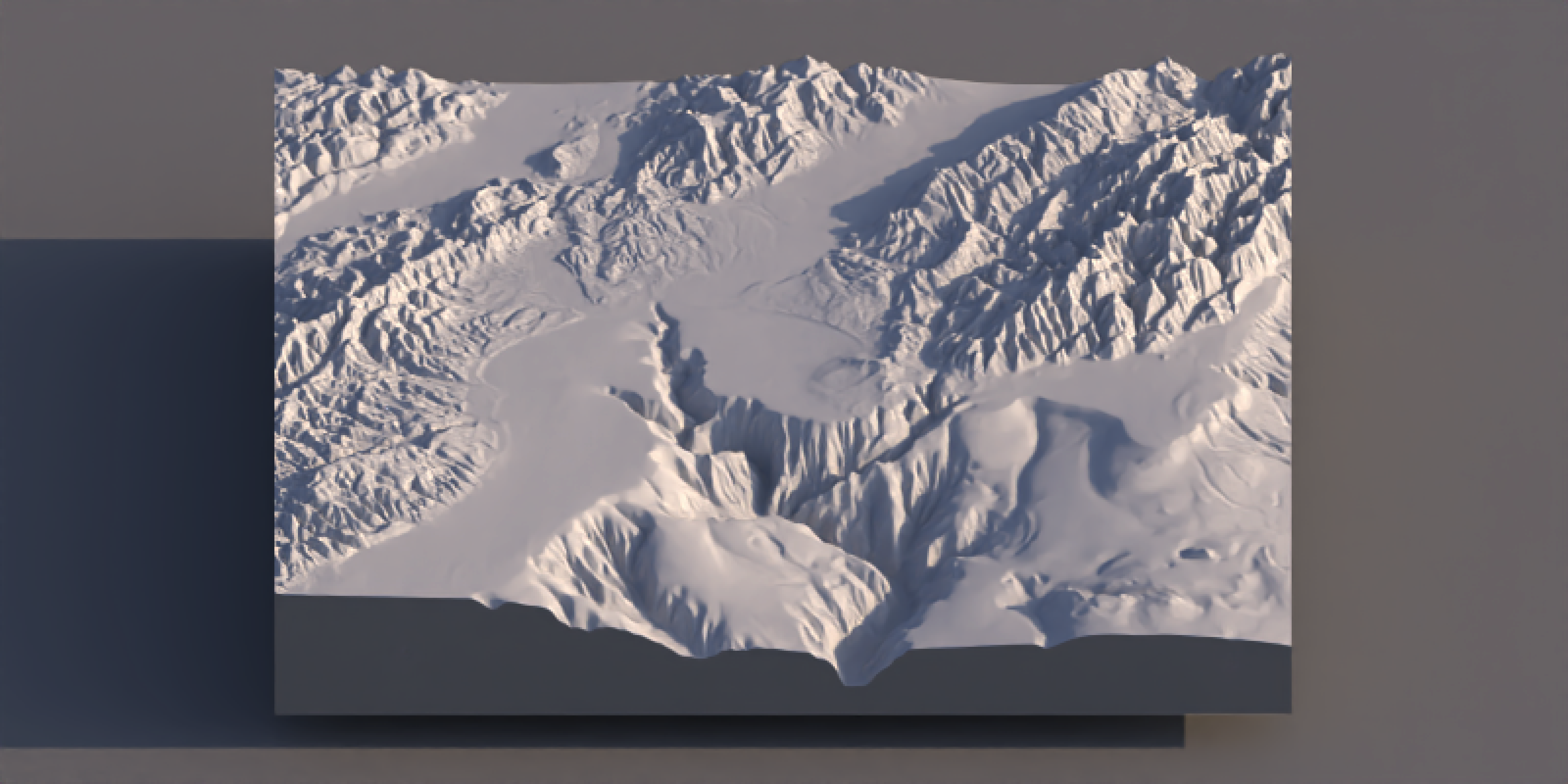
render_monterey("demo_sky.exr", iso = 30) |>
plot_image() 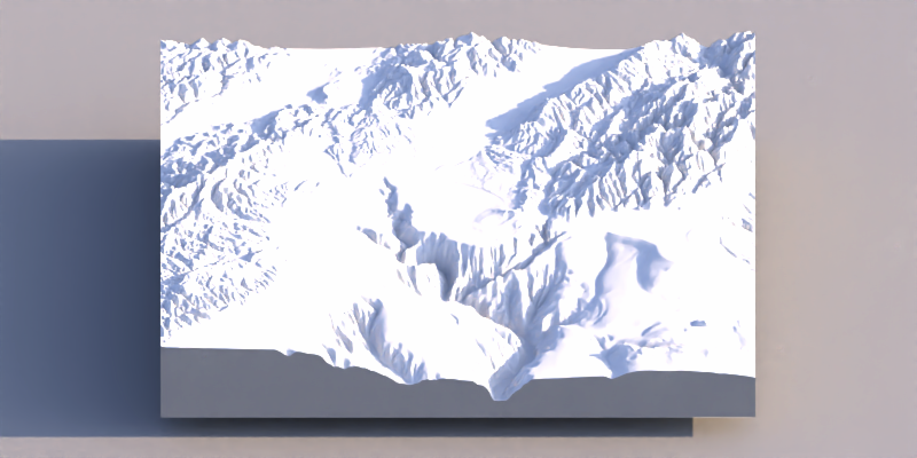
render_monterey("demo_sky.exr", iso = 100) |>
plot_image() 
Two models: Hosek and Prague
Speaking of multiple options, skymodelr provides both the Hosek (2013) atmosphere model and the newer Prague (2022) model. The Hosek model is less accurate, but useful because it doesn’t require any additional downloads and can live on the CRAN as-is; the Prague model needs to download some coefficient tables to function (107 MB ground-level only, 574 MB ground-level wide spectral range, and 2.4 GB for the full altitude model). Those aren’t included in the package by default but will be downloaded as needed when you first call the function, and are cached so they only need to be downloaded once.
Code
demo_sky_sunset = generate_sky(
  elevation = 1, azimuth = 270,
  hosek = TRUE, visibility = 120, albedo = 1,
  resolution = 800, number_cores = 8,
  filename = "demo_sky_sunset.exr"
)
mb_subset = render_monterey("demo_sky_sunset.exr", iso = 80, samples = 32)
plot_image_grid(list(render_exposure(demo_sky_sunset, -6),
                     mb_subset), dim = c(1, 2))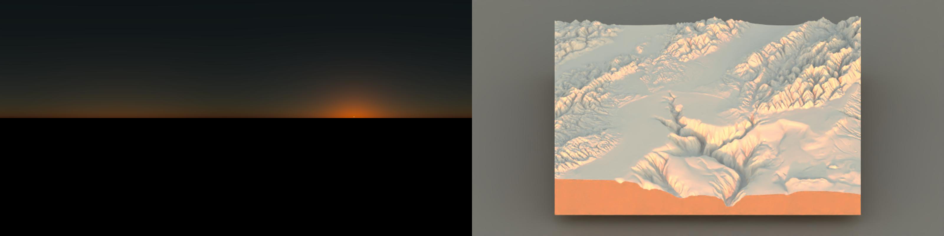
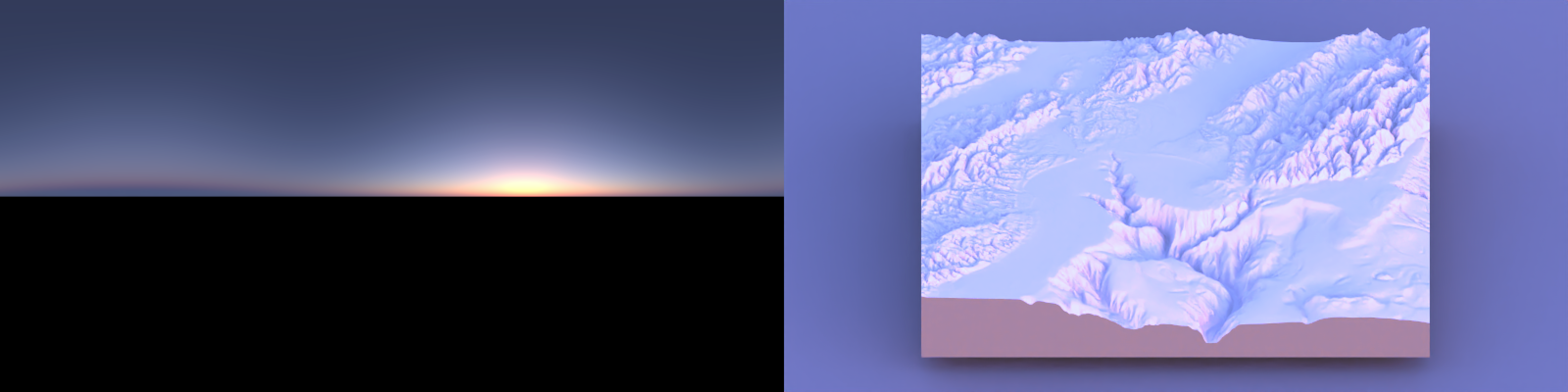
Code
demo_sky_sunset = generate_sky(
  azimuth = 270,   elevation = 1,
  hosek = FALSE, visibility = 120, albedo = 1,
  resolution = 800, number_cores = 8,
  filename = "demo_sky_sunset.exr"
)
mb_subset = render_monterey("demo_sky_sunset.exr", iso = 100, samples = 32)
plot_image_grid(list(render_exposure(demo_sky_sunset, -4),
                     mb_subset),dim = c(1, 2))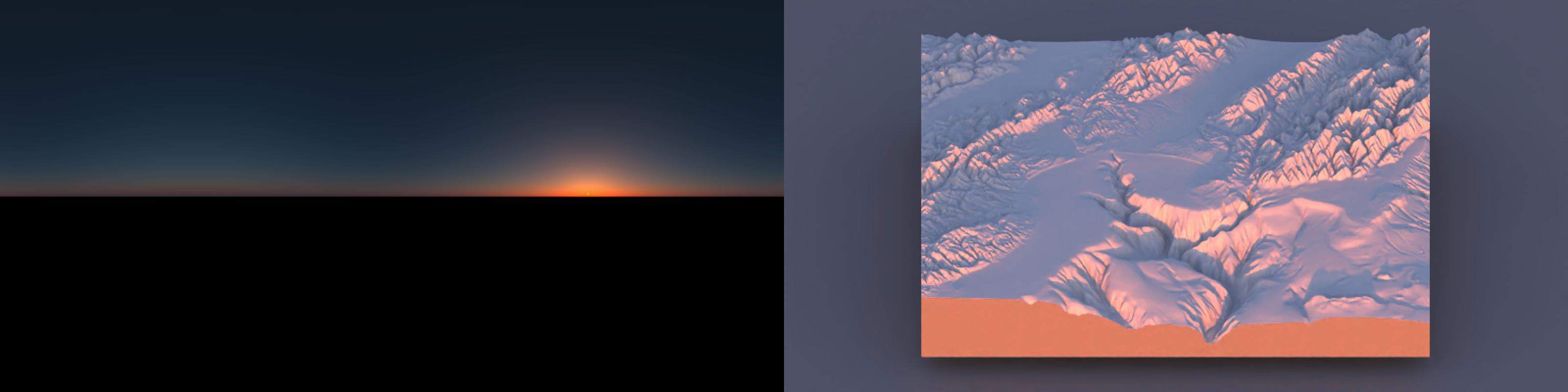
Code
demo_sky_daytime = generate_sky(
  azimuth = 270, elevation = 45,
  hosek = TRUE, visibility = 120, albedo = 1,
  resolution = 800, number_cores = 8,
  filename = "demo_sky_daytime.exr"
)
mb_subset_day = render_monterey("demo_sky_daytime.exr", iso = 100, samples = 32)
plot_image_grid(list(render_exposure(demo_sky_daytime, -6),
                     render_exposure(mb_subset_day,-4)),dim = c(1, 2))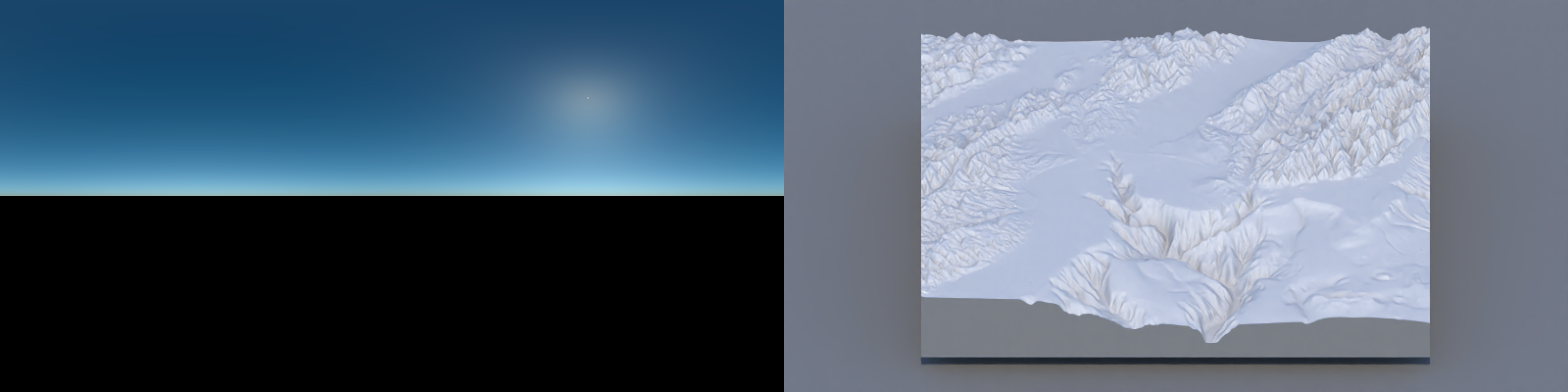
Code
demo_sky_daytime2 = generate_sky(
  azimuth = 270, elevation = 45,
  hosek = FALSE, visibility = 120, albedo = 0,
  resolution = 800, number_cores = 8,
  filename = "demo_sky_daytime2.exr"
)
mb_subset_day2 = render_monterey("demo_sky_daytime2.exr", iso = 100, samples = 32)
plot_image_grid(list(render_exposure(demo_sky_daytime2, -6),
                     render_exposure(mb_subset_day2, -4)),dim = c(1, 2))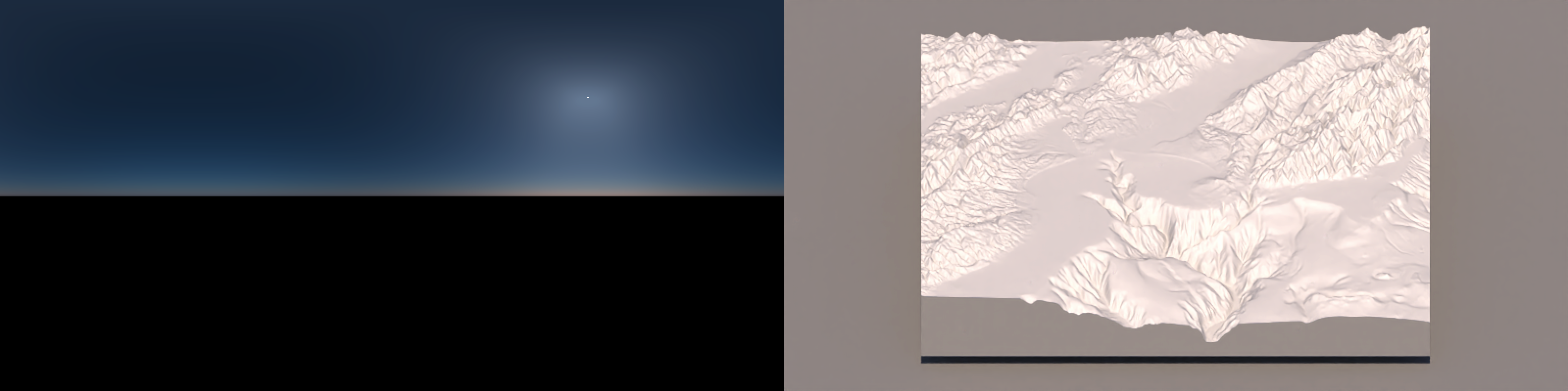
For sea-level renders, the major difference between the two models is the color accuracy: the Hosek daytime colors are just a little too blue, while the sunset is just a little too yellow.
In addition to accuracy, the Prague model adds in some cool features: most notably that it allows you to simulate the atmosphere up to an altitude of 15,000 meters. At those heights you are actually above the bulk of the atmosphere, and thus most of the scattered blue light of the sky is actually coming from below you. The resulting render feels much more like “space” than sky. The scene at 10,000 meters below will also be familiar if you’ve ever flown (and failed to sleep) on a red-eye: the appearance of the sunrise/sunset at 30,000 ft is distinctively different than at ground level.
Code
demo_sky_45_1000 = generate_sky(resolution = 800, azimuth = 225, hosek = FALSE,
                               visibility = 120, altitude = 1000,
                               albedo = 1 , number_cores = 8,
                               elevation = 45)

render_exposure(demo_sky_45_1000, -7, preview=TRUE)
demo_sky_1_1000 = generate_sky(resolution = 800, azimuth = 225, hosek = FALSE,
                               visibility = 120, altitude = 1000,
                               albedo = 1 , number_cores = 8,
                               elevation = 1)

render_exposure(demo_sky_1_1000, -5, preview=TRUE)
Code
demo_sky_45_5000 = generate_sky(resolution = 800, azimuth = 225, hosek = FALSE,
                               visibility = 120, altitude = 5000,
                               albedo = 1 , number_cores = 8,
                               elevation = 45)

render_exposure(demo_sky_45_5000, -7, preview=TRUE)
demo_sky_1_5000 = generate_sky(resolution = 800, azimuth = 225, hosek = FALSE,
                               visibility = 120, altitude = 5000,
                               albedo = 1 , number_cores = 8,
                               elevation = 1)

render_exposure(demo_sky_1_5000, -5, preview=TRUE)

Code
demo_sky_45_10000 = generate_sky(resolution = 800, azimuth = 225, hosek = FALSE,
                                 visibility = 120, altitude = 10000,
                                 albedo = 1 , number_cores = 8,
                                 elevation = 45)

render_exposure(demo_sky_45_10000, -7, preview=TRUE)
demo_sky_1_10000 = generate_sky(resolution = 800, azimuth = 225, hosek = FALSE,
                                visibility = 120, altitude = 10000,
                               albedo = 1 , number_cores = 8,
                               elevation = 1)

render_exposure(demo_sky_1_10000, -5, preview=TRUE)

Code
demo_sky_45_15000 = generate_sky(resolution = 800, azimuth = 225, hosek = FALSE,
                                 visibility = 120, altitude = 15000,
                                 albedo = 1 , number_cores = 8,
                                 elevation = 45)

render_exposure(demo_sky_45_15000, -7, preview=TRUE)
demo_sky_1_15000 = generate_sky(resolution = 800, azimuth = 225, hosek = FALSE,
                                visibility = 120, altitude = 15000,
                                albedo = 1 , number_cores = 8,
                                elevation = 1)

render_exposure(demo_sky_1_15000, -5, preview=TRUE)

Lighting real world places with rayshader
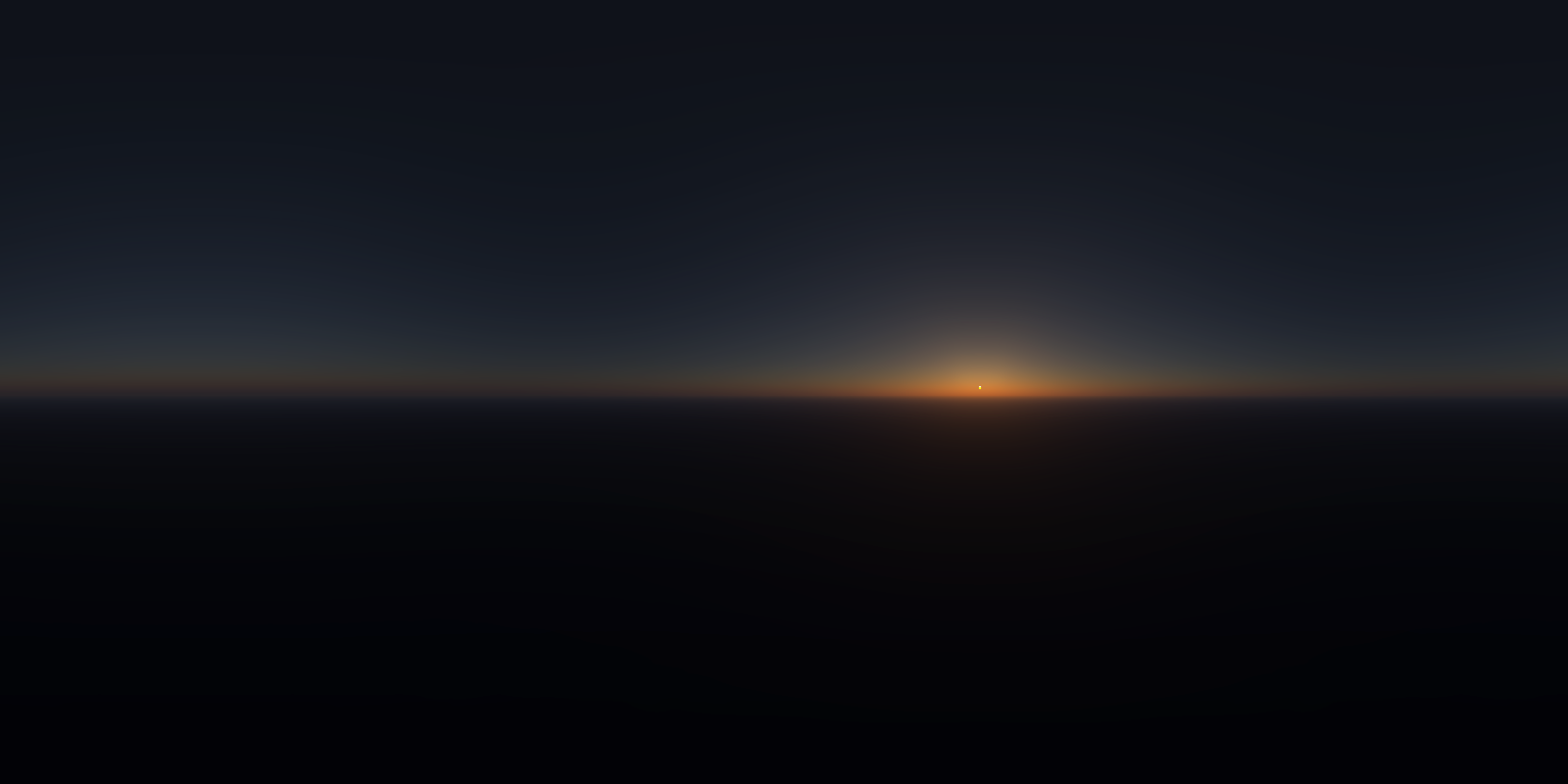
We also get a very practical use from this package elsewhere in the rayverse: we can now generate realistically lit landscapes in rayshader with just a latitude, longitude, and date and time! skymodelr implements this in the function generate_sky_latlong. Instead of manually specifying an azimuth and elevation for our sun, we just pass in a location and time, and skymodelr will use the suncalc package to calculate the sun’s elevation and azimuth in the sky. This allows us to generate accurate depictions of how shadows fall across real-world places, taking into account both direct sunlight as well as indirect atmospheric scattered lighting. The latter is critical for rendering dramatic terrain: for example, visualizing lighting in deep valleys or between skyscrapers.
As an example, let’s look at the difference between the Rio Grande gorge in New Mexico, as seen right after sunrise (specifically, around 6:20 AM in mid-July, since that’s where I found some good reference photographs with a specified date and time). We’ll visualize it three ways: first, with just a simple sphere representing the sun, then with a carefully colored sphere with a blue/white gradient sky, and then with the full atmospheric model:
Code
center_lon = -105.7334
center_lat = 36.4756
datetime_sunrise = as.POSIXct("2025-07-22 06:15:00", tz="America/Denver")

d = 0.005
aoi = st_as_sfc(st_bbox(c(
  xmin = center_lon - d, ymin = center_lat - d,
  xmax = center_lon + d, ymax = center_lat + d
), crs = 4326))

aoi_sf = st_sf(geometry = aoi)

bbox_ll = st_bbox(aoi)

q_waterway = opq(bbox = bbox_ll, timeout = 240) |>
  add_osm_feature(key = "waterway")
Sys.sleep(1)

osm_waterway = osmdata_sf(q_waterway)
water_lines = osm_waterway$osm_lines

aoi_utm = st_transform(aoi_sf, 32613)
water_lines_utm = st_transform(water_lines, 32613)
dem = get_elev_raster(locations = aoi_sf, z = 14, src = "aws" )
dem_t = rast(dem)

# UTM 13N covers Taos/Rio Grande Gorge area
dem_utm = project(dem_t, "EPSG:32613", method = "bilinear", res = 10)
dem_utm = trim(dem_utm)
dem_r = raster(dem_utm)
elmat = raster_to_matrix(dem_r) |>
  rayimage::render_resized(mag=5) |>
    (\(x) {
    x[is.na(x)] = NA
    x
  })()

water_overlay = generate_line_overlay(
  geometry = water_lines_utm,
  extent = raster::extent(dem_r),
  heightmap = elmat,
  color = "deepskyblue2",
  linewidth = 10
)

tex = elmat |>
  sphere_shade(texture = "imhof4") |>
  add_overlay(water_overlay, alphalayer = 0.9)

sunpos = suncalc::getSunlightPosition(
  lat = center_lat,
  lon = center_lon,
  date = datetime_sunrise
)[c("altitude","azimuth")]*180/pi


demo_sky_sunset_nm = generate_sky_latlong(
  lat = center_lat, lon = center_lon,
  datetime = datetime_sunrise,
  resolution = 1600, hosek = FALSE, visibility = 120, altitude = 0, verbose = TRUE,
  albedo = 1, number_cores = 8, filename="demo_sky_sunset_nm.exr"
)

plot_3d(
  hillshade = tex,
  heightmap = elmat,
  zscale = 2,
  solid = TRUE,
  shadow = TRUE,
  windowsize = c(800, 600),
  theta = 315, phi = 40,
  zoom = 0.75, fov = 70
)

constant_shade(matrix(1,100,100), color = "lightblue") |>
  rayimage::ray_write_image("lightbluesky.png")

lookfrom = c(-208.69, 58.10, 870.62)
lookat = c(514.54, -80.26, -1624.73)


render_highquality(
  sample_method = "sobol",
  clamp_value = 10000,
  lightaltitude = sunpos[["altitude"]],
  lightdirection = 180+sunpos[["azimuth"]],  #suncalc measures from south
  lightsize = 100,
  lightintensity = 10000,
  camera_location = lookfrom, camera_lookat = lookat, aperture=0,
  width = 800, height=600, #preview = FALSE, plot = TRUE,
  cache_scene = TRUE
)
render_highquality(
  sample_method = "sobol",
  clamp_value = 1000,
  lightaltitude = sunpos[["altitude"]],
  lightdirection = 180+sunpos[["azimuth"]],
  lightsize = 100,
  lightcolor = "#ff7403",
  lightintensity = 20000,
  ambient_light = TRUE,
  backgroundlow="white", backgroundhigh = "#3C4B6B",
  camera_location = lookfrom, camera_lookat = lookat, aperture=1,
  width = 800, height=600, preview = FALSE, plot = TRUE, cache_scene = TRUE
)
render_highquality(
  sample_method = "sobol",
  clamp_value = 1000,
  light=FALSE,
  environment_light = "demo_sky_sunset_nm.exr", iso = 25,
  camera_location = lookfrom, camera_lookat = lookat, aperture=1,
  width = 800, height=600, preview = FALSE, plot = TRUE, cache_scene = TRUE
)
rgl::close3d()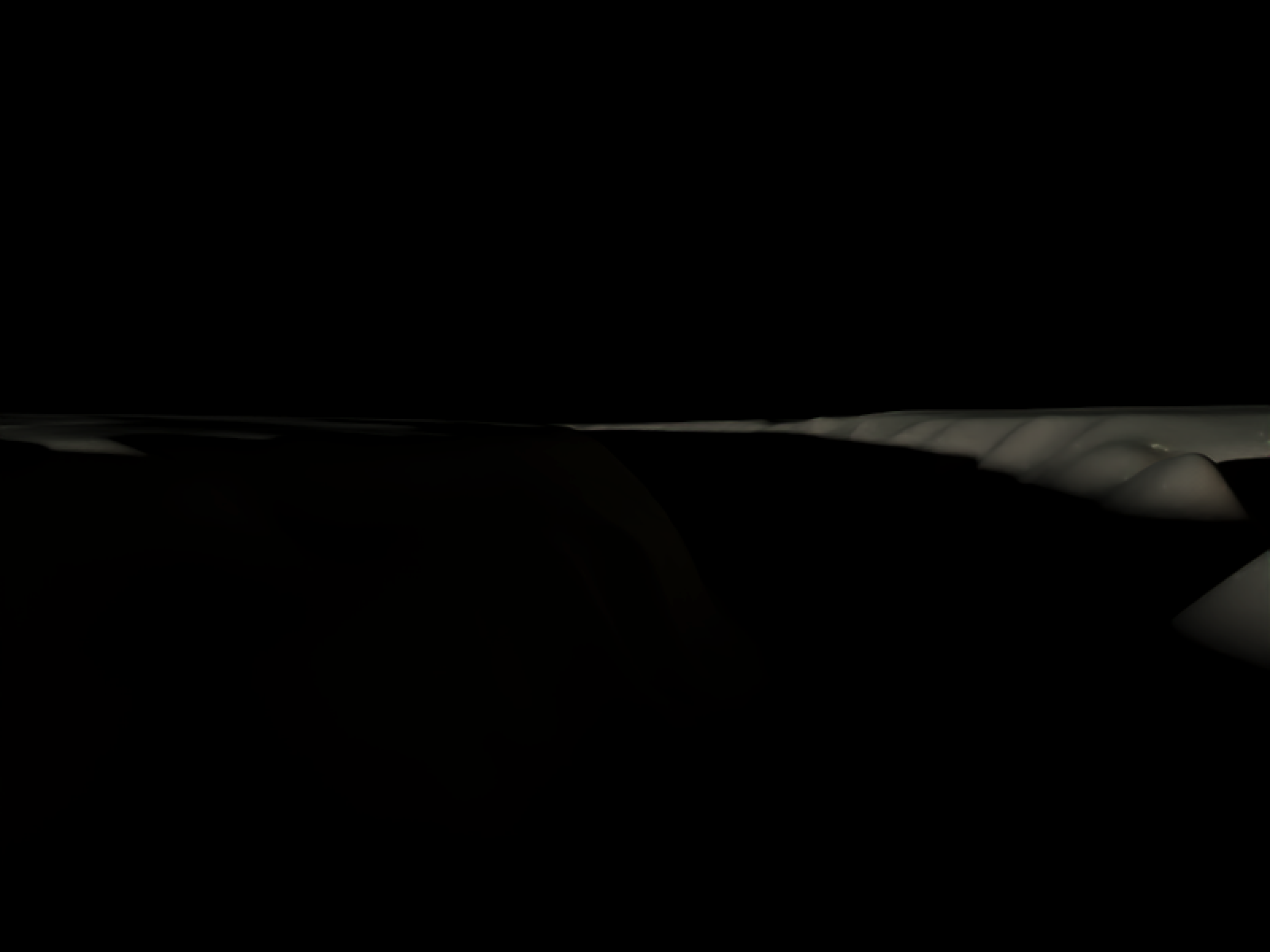
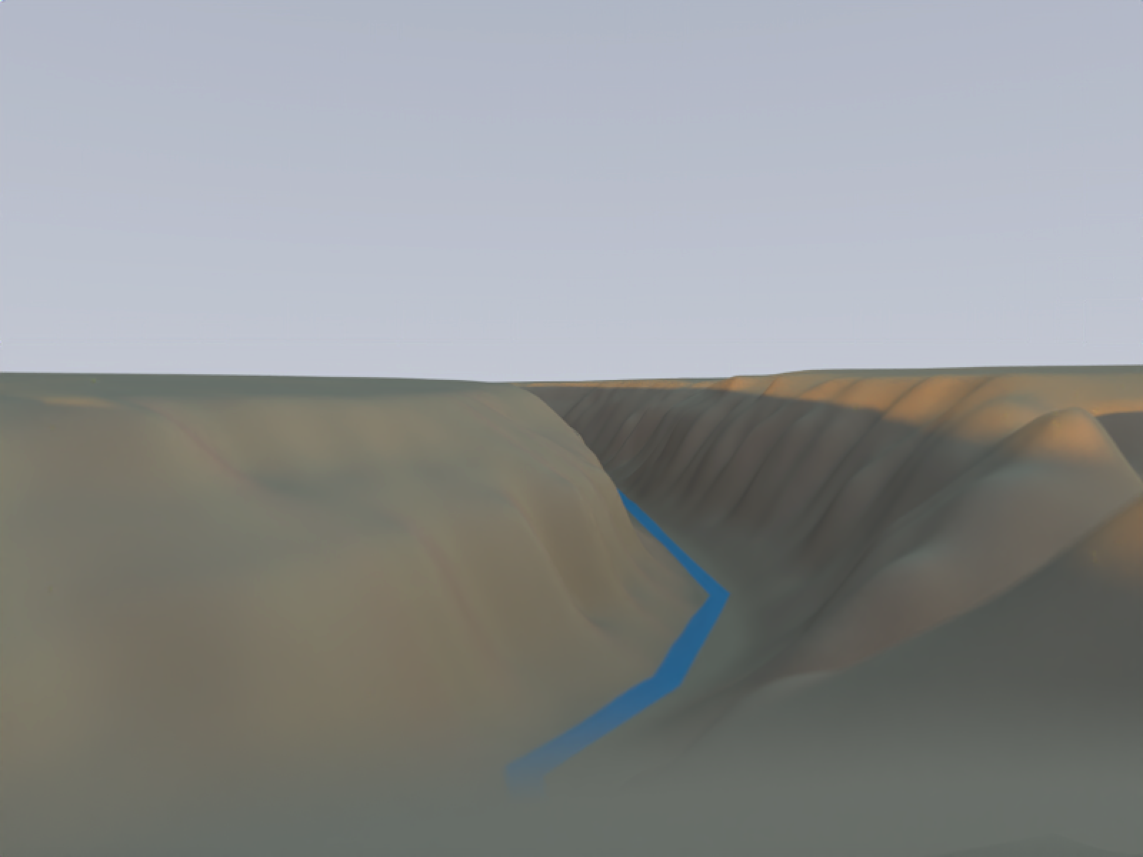
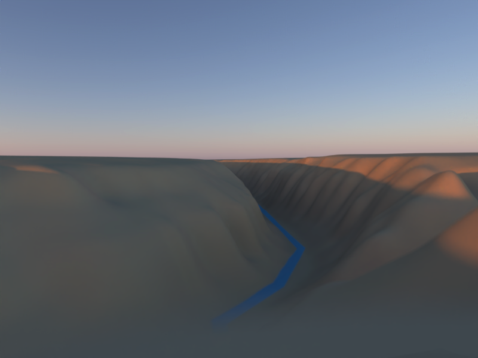
It’s clear above that the single light version isn’t going to cut it with this type of terrain: we need indirect lighting from the atmosphere to light up dramatic terrain like this. The middle version is passable as an overcast day, but it’s not very visually interesting. The right version? Makes me want to grab a coffee and enjoy a crisp desert morning in a national park.
One nice thing about the newer Prague atmospheric model is that it actually allows us to model the atmosphere when the sun is below the horizon. This allows us to render spaces with the really nice color gradient of a sunset without any harsh direct lighting at all. We can also use the rayimage package to perform some stylistic color transformations on the render (white balance adjustments/saturation tweaks) to make the color contouring more obvious.
Code
sky_after_sunset = generate_sky_latlong(
  lat         = 38.9072,
  lon         = -77.0369,
  datetime = as.POSIXct("2025-12-29 16:59:00", tz = "EST"),
  resolution = 800, hosek = FALSE, visibility = 120,
  albedo = 1 , number_cores = 8, verbose = TRUE,
  filename="sky_after_sunset.exr"
)

mb_sunset = render_monterey("sky_after_sunset.exr", iso=1000, samples = 32)
mb_custom_style = mb_sunset |>
  render_white_balance(target_white = "D50") |>
  render_vibrance(vibrance = 0.25,protect_luminance = 0.10) |>
  render_exposure(0.3)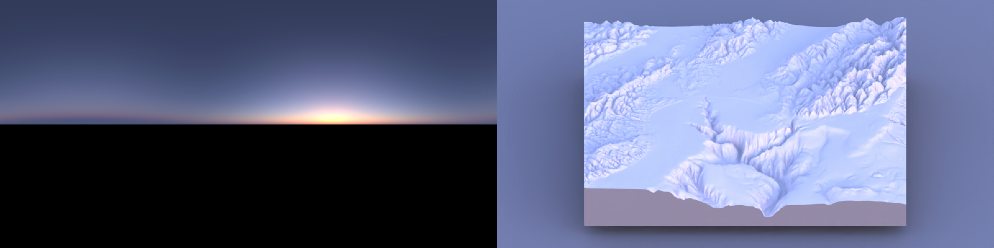
However, if we don’t care about adhering to the pesky rules of physics, these models also allow us to cheat: we can generate a sky that has all the scattered skylight, but doesn’t include the direct contribution from the sun’s disk.
Code
sky_midday = generate_sky_latlong(
  lat      = 38.9072,
  lon      = -77.0369,
  datetime = as.POSIXct("2025-06-21 15:00:00", tz = "EST"),
  resolution = 800, hosek = FALSE, visibility = 120,
  albedo = 0 , number_cores = 8, verbose = TRUE,
  render_mode = "atmosphere",
  filename="sky_midday.exr"
) |>
  render_exposure(-5)

mb_midday = render_monterey("sky_midday.exr", iso=40, samples = 32)

plot_image_grid(list(sky_midday, mb_midday), dim=c(1,2))
My opinion? It’s okay. Not as good as the sunset, due to the overbearing blueness. But you’ll notice the same thing in real life if you carefully look at objects in shadow under the midday sun: everything has a slight blue cast to it that your eyes do a good job “color correcting” away.
Now that we can generate our artificial skies, we can move on to the next challenge: how do we properly integrate them into our 3D scenes to represent real places? We have a 3D model that represents a real location and we have to ensure that the sky coordinate system and the geospatial coordinate system align. Basically, we need the XZ axis in our 3D model to align with our environment map orientation. How do we do that? Well, one way to solve it is to just tell people to stick with one convention for the direction of North, for all maps, until the heat death of the universe. North is +Z and East is +X.3
There, wasn’t that easy? I take it back–the cartographer Illuminati had the right idea. So much easier (for me).4
Examples
That’s enough about how it works. Let’s see the package in action: lighting actual 3D scenes.
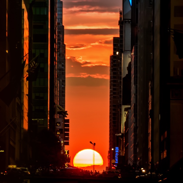
Manhattanhenge
To stress test the package, let’s choose a rather difficult example that requires a precise alignment between geospatial data and the sun to observe: Manhattanhenge! Also called the “Manhattan Solstice,” it’s a cosmic alignment between the east–west grid of New York City and the setting sun that occurs a few times a year.
This is a particularly challenging problem because not only do the terrain and sky need to be aligned, but so do the building footprints: we’re trying to seamlessly combine three separate datasets: sky, ground, and polygon. It’s a good integrated test of rayshader’s render_polygons()/render_buildings() logic. Let’s fly through the streets of Manhattan and see how well it lines up:
Code
planar_crs = "EPSG:32118" # or 32618
lower_man_bbox = c(
xmin = -73.958,
ymin = 40.757,
xmax = -74.005,
ymax = 40.77
)
q = opq(
bbox = c(
lower_man_bbox["xmin"],
lower_man_bbox["ymin"],
lower_man_bbox["xmax"],
lower_man_bbox["ymax"]
)
) |>
add_osm_feature(key = "building")
osm = osmdata_sf(q)
bldg_polys = bind_rows(
osm$osm_polygons |>
dplyr::select(any_of(c("building", "height", "building:levels")), geometry),
osm$osm_multipolygons |>
dplyr::select(any_of(c("building", "height", "building:levels")), geometry)
) |>
st_make_valid()
lower_man_poly = st_as_sfc(
st_bbox(lower_man_bbox, crs = 4326)
)
parse_height_numeric = function(x) {
x_num = gsub("[^0-9\\.]", "", x)
as.numeric(x_num)
}
bldg_polys = bldg_polys |>
mutate(
height_m = parse_height_numeric(height),
levels = suppressWarnings(as.numeric(`building:levels`)),
height_m = case_when(
!is.na(height_m) ~ height_m,
is.na(height_m) & !is.na(levels) ~ levels * 3,
TRUE ~ NA_real_
)
) |>
filter(!is.na(height_m)) |>
filter(height_m < 1000)
bldg_polys = bldg_polys |>
mutate(top_height = height_m)
lower_man_poly_planar = st_transform(lower_man_poly, planar_crs)
bldg_polys_planar = bldg_polys |>
st_make_valid() |>
st_transform(planar_crs)
ll_proj = "+proj=longlat +datum=WGS84 +no_defs"
bb = st_bbox(lower_man_poly)
loc_df = data.frame(
x = c(bb["xmin"], bb["xmax"]),
y = c(bb["ymin"], bb["ymax"])
)
dem_raster = get_elev_raster(
locations = loc_df,
z = 13,
prj = ll_proj,
clip = "bbox"
)
dem_raster_planar = rast(dem_raster)
crs(dem_raster_planar) = "EPSG:4326"
dem_raster_planar = project(dem_raster_planar, planar_crs, method = "bilinear")
dem_raster_planar = crop(
dem_raster_planar,
terra::vect(lower_man_poly_planar)
)
lower_man_vect = terra::vect(lower_man_poly_planar)
dem_raster_planar = terra::crop(dem_raster_planar, lower_man_vect)
bbox_planar = sf::st_bbox(lower_man_poly_planar)
dem_raster_planar = terra::crop(
dem_raster_planar,
terra::ext(
bbox_planar["xmin"],
bbox_planar["xmax"],
bbox_planar["ymin"],
bbox_planar["ymax"]
)
)
# 4. Convert DEM to matrix for rayshader
elev_mat = raster_to_matrix(dem_raster_planar)
# 5. Build a base shaded relief map
zscale = 10
hillshade = sphere_shade(elev_mat)
# 6. Plot 3D terrain with rayshader
hillshade |>
plot_3d(
elev_mat,
zscale = 10,
fov = 0,
theta = -45,
phi = 45,
zoom = 0.75,
background = "black",
windowsize = c(1200, 900)
)
# 7. Extrude buildings with render_buildings()
render_polygons(
polygon = bldg_polys_planar,
extent = dem_raster_planar,
heightmap = elev_mat,
data_column_top = "top_height",
data_column_bottom = NULL,
scale_data = 1 / 10,
color = "grey20",
clear_previous = TRUE
)
render_camera(fov = 8)
skymodelr::generate_sky_latlong(
lat = 40.7128,
lon = -74.0060,
altitude = 0,
resolution = 6000,
hosek = FALSE,
number_cores=8,
datetime = as.POSIXct("2022-05-29 20:13:00", tz = "America/New_York"),
filename = "manhattan_alignment.exr"
)
render_highquality(
iso = 15,
preview = TRUE,
sample_method = "sobol",
environment_light = "manhattan_alignment.exr",
light = FALSE,
width = 800,
height = 800,
samples = 256,
clamp_value = 10000,
aperture = 0,
camera_location = c(143.73, -18.01, 24.96),
camera_lookat = c(-7107.84, -25.85, -3979.55),
override_material = TRUE,
material = rayrender::glossy(color="grey50",gloss = 0.6,reflectance = 0.01)
)- 1
- Rough extent for Lower Manhattan
- 2
- Get building footprints + height from OSM
- 3
- Combine polygons + multipolygons into a single sf object
- 4
- sf polygon for the bbox (WGS84)
- 5
- Derive/approximate building height in meters
- 6
- Column for rayshader to use as building top height
- 7
- Reproject building polygons
- 8
- Get and prep Manhattan terrain data
- 9
- Plot base rayshader map
- 10
- Plot buildings
- 11
- Generate sky EXR
- 12
- Render single frame of pathtracer scene
Look at that–it’s aligned! The sun is squarely in the middle of the road and partly under the horizon at May 29th, 2022 at 8:13 p.m., which matches the time listed in the table on the Manhattanhenge Wikipedia page for the half-sun time.
The Staff of Ra(ytracing)
The successful celestial alignment of Manhattanhenge is a nice example suggesting correctness, but it’s just one data point. I’ve run into situations where an algorithm looks correct in an initial test, but that success is just the result of two errors canceling out, and subsequent tests fail. For example, I could imagine some issue with both the building polygon projection and the sky calculation that happens to align. So let’s offer another, more convincing example, inspired by a film series that made precise alignment of the sun and a model into a critical plot point: Indiana Jones.
In Raiders of the Lost Ark, there’s a whole sequence where they have to find the fictional “Staff of Ra” to uncover the location of the Ark. Indiana eventually ends up in the ancient Egyptian equivalent of a model train enthusiast’s basement, where the precise alignment of the sun and the jewel on the rod sends a beam that reveals the location of the Ark.5
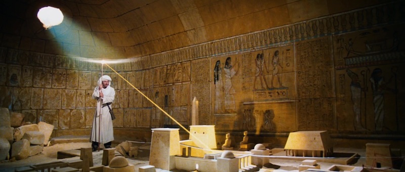
This was a lot of work that could be saved if Indy had an accurate atmospheric radiance model, along with a highly accurate digital model of the archaeological site. And would you know it: there are organizations around today with the explicit mission of digitizing historical sites in 3D! The Global Digital Heritage is an organization devoted to documenting the world’s cultural and natural history, and has digitally preserved many historical sites with detailed 3D scans with geospatial accuracy in mind. And one of the places recently scanned (in November 2024) was most famously featured in “Indiana Jones and the Last Crusade” as the entrance to the site that holds the Holy Grail: Al-Khazneh in Petra, Jordan (“The Treasury” in English).
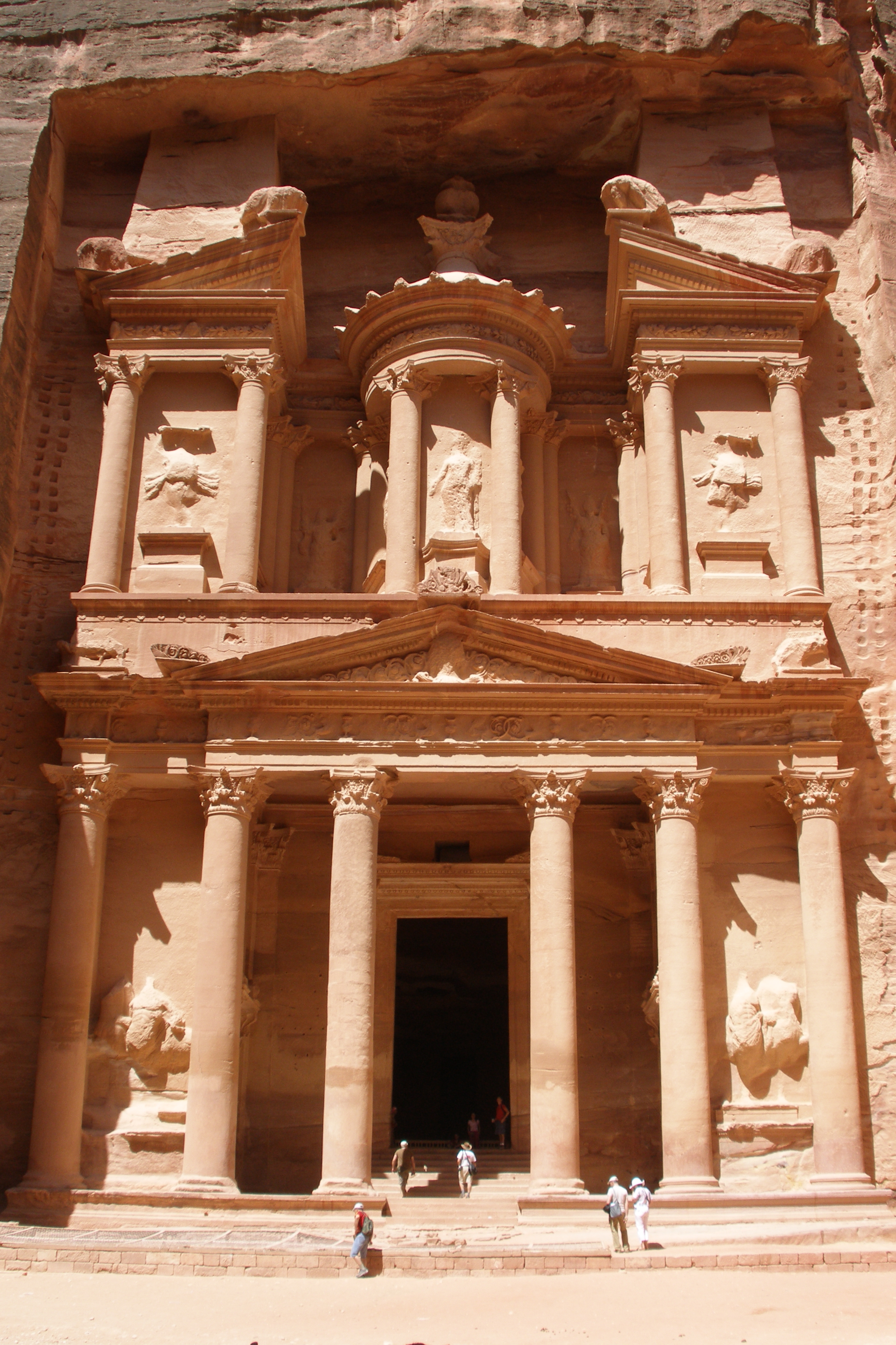
One nice trait of such a famous, well-known location is that you can find hundreds (if not thousands) of photos of said location, freely available on Wikimedia Commons, such as the one above. Complete with full metadata. Including the exact date and time that the photo was taken. So we can pick a photo and pull the time it was taken, which along with the lat/long of Al-Khazneh should give us a good golden test of our atmospheric model. We’ll display the render alongside the image and see how the shadows compare.
lat_treasury = 30.328960
long_treasury = 35.444832
skymodelr::generate_sky_latlong(
lat = lat_treasury,
lon = long_treasury,
altitude = 1000,
resolution = 2000,
hosek = FALSE,
number_cores=8,
datetime = as.POSIXct("2007-06-03 10:17:57", tz = "Asia/Amman"),
filename = "Al_Khazneh.exr"
)
obj_model("al-khazneh-petra-jordan/source/treasury/Al-Khazneh.obj",
angle = c(-90,0,0)) |>
render_scene(
lookfrom=c(39.13, 2.23, -16.72),
lookat= c(2.74, 19.74, 2.19) ,fov=52.4,
width=2048,height = 3072, samples = 32,
aperture=0.00, iso=3,
filename = "treasury.exr",
environment_light = "Al_Khazneh.exr"
)
render_exposure("treasury.exr",1) |>
render_white_balance(reference_white = "D75",
target_white = "D50",
bake = TRUE) |>
ray_write_image("rendered_treasury.exr")- 1
- Time taken from the EXIF data of the photograph
- 2
- The data uses +Z as the up direction, so we rotate it \(90^\circ\) around the X axis to make +Y up
- 3
- The original photo’s white balance is unknown, so I baked in a manual adjustment to make the photo’s color appear closer
Figure 23 shows that the shadow outlines are pretty spot on, with only minor differences due to the precision of the 3D model. Success!
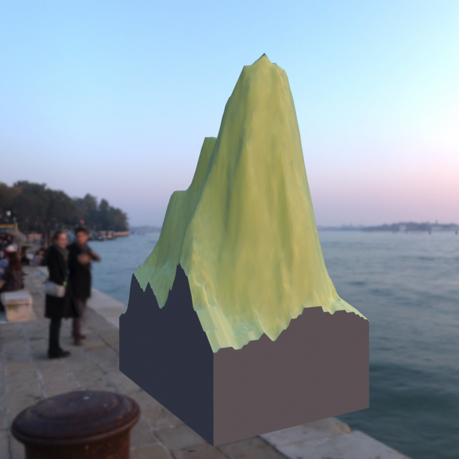
Abstract dataviz
Now that we’re done probing the package’s ability to generate realistic spatial scenes, let’s see if it provides nice lighting for a purely abstract visualization. We’ll try it out with a 3D ggplot from rayshader, using my favorite 3D ggplot demo: a faceted 3D density plot of the diamonds dataset.
Code
library(ggplot2)
library(viridis)

ggdiamonds = ggplot(diamonds, aes(x, depth)) +
 stat_density_2d(aes(fill = after_stat(nlevel), color = after_stat(nlevel)),
                 geom = "polygon",
                 n = 200, bins = 50,contour = TRUE) +
 facet_wrap(clarity~.) +
 scale_fill_viridis_c(option = "A") +
 scale_color_viridis_c(option = "A")

plot_gg(ggdiamonds,width=5,height=5,scale=250,windowsize=c(1200,600),
        raytrace = FALSE, theta = 30, phi = 30, zoom = 0.33, fov = 50)

generate_sky(
  elevation = 2, azimuth=315,
  resolution = 1600, hosek = FALSE, visibility = 120, altitude = 0, verbose = TRUE,
  albedo = 1, number_cores = 8, filename="demo_sky_sunset2.exr"
)

render_highquality(
  sample_method = "sobol",
  clamp_value = 1000,
  light=FALSE,
  environment_light = "demo_sky_sunset2.exr", iso = 50,
  aperture=1,
  width = 1200, height=600, preview = FALSE, plot = TRUE, cache_scene = TRUE,
  rotate_env = 270,camera_lookat=c(0,-100,0)
)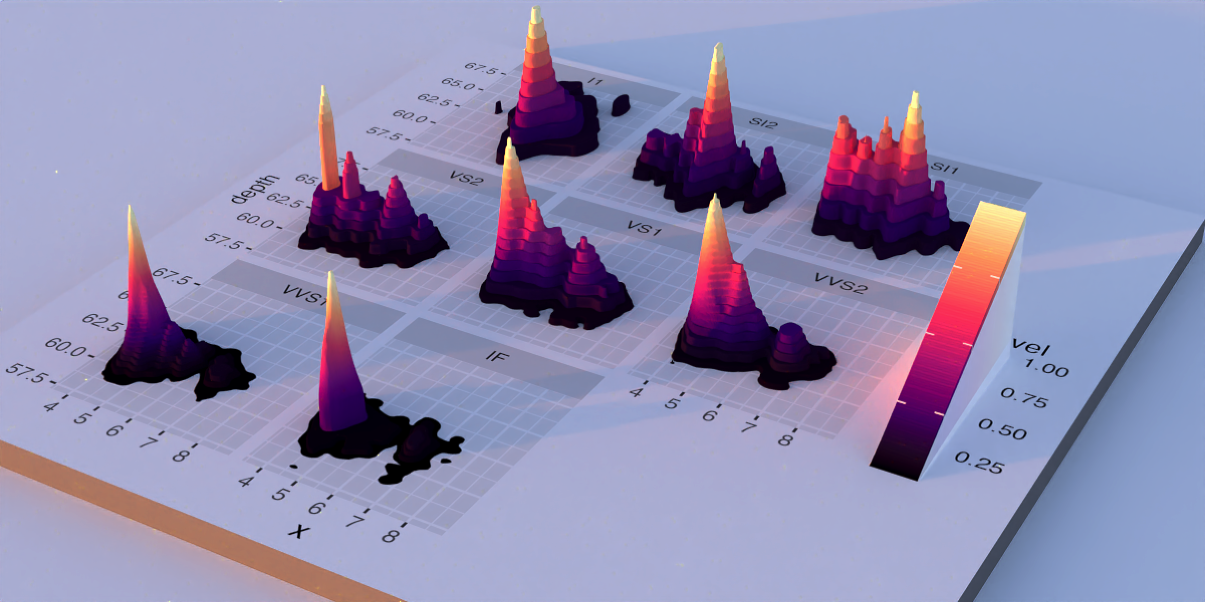
Soft shadows, nice highlights, good color: 8/10! Why not 10/10 on my entirely subjective self-assessment? Well, there are definitely some changes I would make if I were really focused on “perfecting” the lighting here: I’d punch up the key light and increase the solar angle so the shadows weren’t so long. But these are nitpicks, and the raw solar atmospheric simulation of sunset provides a solution that’s good enough for most purposes–and that’s the point! We can get the 80% “good enough” solution and focus our energy on the actual 3D data.
Using it in rayshader
lat/long/datetime in render_highquality()
Since programmatically generating a realistic atmosphere that matches the ideal conditions for a place and time is so obviously such a cool feature, I’ve made it easy to do in R via rayshader: rather than having the user manually generate an EXR file with skymodelr, I added several new arguments to render_highquality() to do it for you: lat, long, datetime, and sky_args. These arguments generate the EXR file for you and add it to the scene (along with turning off the default light), so you don’t have to manually pipe in the environment light.
montereybay |>
sphere_shade() |>
plot_3d(montereybay, water=TRUE,
theta = 0, fov = 0, zoom = 1)
for (i in seq_len(100)) {
set.seed(1)
render_highquality(
long = -121.866,
lat = 36.679,
datetime = as.POSIXct("2026-02-01 07:15:00", tz = "America/Los_Angeles") +
lubridate::duration(6 * i, "minutes"),
samples = 64,
sample_method = "sobol",
iso = 5,
clamp_value = 100,
sky_args = list(hosek = FALSE, resolution = 4000, number_cores = 8),
filename = sprintf("nodenoise_mb%d.exr", i),
denoise = FALSE
)
}- 1
- New arguments.
- 2
- Note: We turn off OIDN denoising because it can cause flickering: denoising doesn’t accurately preserve the brightness from frame to frame.
Think of the possibilities: want to visualize the impact of a new skyscraper’s shadow on nearby parks, taking into account the loss of direct sunlight as well as scattered light? Easy. Find great alignments between the terrain and sunsets for awesome photographs? Lat + long + datetime = done. Map the shadiest route through a city during a hot summer day at a particular date and time?6 Don’t sweat it, we’ve got you covered.
It’s skymodelr, not daymodelr
However, after all of these cool features, there’s still a problem: when the sun drops below the horizon (more than \(4^\circ\) below the horizon for the Prague model), our simulated sky is black. Not because the model says so: rather, the model simply isn’t valid. And if you go out and look up at the sky at night, you will notice very clearly that the sky isn’t uniformly black. And the name of the package is skymodelr, and yet we aren’t modeling the sky about 50% of the time.
This is not ideal. Doubly so because passing a uniformly black EXR as a background image can cause computational issues in a pathtracer if you aren’t careful, since trying to normalize the sampling distribution (for importance sampling purposes) fails due to division by zero. Is there a way we can also have an accurate model of the night sky as well?
Why, of course!
But this blog post has gone on for long enough: that discussion will have to wait for Part 2 of this blog post, covering realistic rendering of the Moon, the planets, and the stars! In the meantime, you can explore and install the package yourself.
Github

Installation
remotes::install_github("tylermorganwall/skymodelr")Footnotes
You can read a nice blog post all about lighting ratios here that I found informative here.↩︎
But also because it’s R, and canonically you need at least two ways to perform any one task in the language, so we’re too busy infighting (Tidy vs Base! dplyr vs data.table! Base pipe vs magrittr!) to even consider looking at other languages :)↩︎
Just kidding, when I did this I discovered that I had unwittingly followed the OpenGL left-handed convention when setting up my pathtracer’s coordinate system, which meant that +X was to the left (west) when looking towards +Z, which is a big yuck. But it couldn’t be fixed simply by negating the Z axis, since such a negation would flip the “direction” of the surface so it points inwards. So I had to plumb a fix deep into rayrender’s internals and rewrite half of the examples to match this coordinate choice. Chirality bugs: the worst.↩︎
If you are both 1) smart and technically minded and also 2) annoying, you might be considering writing a comment noting that if the center of your map is aligned with one of the Earth’s poles, this convention runs into a coordinate singularity and will fail. Sadly, the landless oceanic void at the north pole and the featureless expanse of snow and ice at the south pole will have to wait for someone who cares… Just kidding! I do care, Mr. More-of-a-comment-than-a-question: I also added an argument to specify the north direction of the 3D model in rayshader, so you can choose your own convention.↩︎
We are supposed to just accept that Indy just happens to get into the map room at exactly the date where the Earth’s axial tilt lines up with the hole leading to the location of the Ark, yet he could have easily shown up on a different date, producing a different location. I mean, what are we to believe, that this is some sort of a magic crystal rod or something? Boy, I really hope somebody got fired for that blunder…↩︎
This is actually something I imagined doing every day in grad school when walking from my apartment to my lab through the humid, Baltimore summer. Every week or so I’d find a good route that would keep me from being drenched in sweat by the time I got to my lab, and every other week the sun would shift just enough that the old route no longer was ideal.↩︎