Learn R #1: There’s no need to apply() yourself.
Do you fall into one of these categories?
Programmer who wants to break into data science:

You’re skilled at Python and data wrangling, but you find the non-machine learning libraries provided by the Python community sometimes limiting. You’ve seen the beautiful plots people are able to create with R, but struggle to recreate them easily in Python with matplotlib. You want the ability to easily analyze data and create professional reports and responsive web dashboards.
Excel power user:

You’re analyzing data and hand-building reports regularly with Excel. You make extensive use of Excel formulas and even automate some of your workflow using Visual Basic. You spend a large amount of time manipulating data and feel like Excel is limiting the quality and speed of your deliverables.
Professional analyst who pays for specialized tools:

You’re using SAS/SPSS/STATA/JMP to analyze data. You or your organization pays a lot of money each year to have access to these tools. You want to expand your skill set to include fewer proprietary tools and get access to cutting edge software without paying for expensive black box tool kits.
This is the first post in my Learn R series: One of the major differences between these posts and my analysis posts is showing all the code I use to create, manipulate, and display the data. The code portions that are critical for the discussion will be shown by default, while those used for generating the plots will be collapsed but expandable. I am only going to assume a basic knowledge of programming–enough to know what a for loop is and how to do basic language-agnostic actions like assigning variables, accessing an index in an array/vector, and calling functions. If you don’t know how to do these things, I would recommend any basic series on learning programming before beginning.
First things first: What is R? R is a powerful open source programming language meant for analyzing data. R is designed by people who analyze data, for people who analyze data. Compare this with Python, which was designed by programmers, for other programmers. Or Perl, which was designed by monkeys randomly pounding on keyboards without alphanumeric characters. It’s a language built for diving deep into data. That’s not to say other languages don’t have this ability, but R is by far the most developed and best supported.
R is designed by people who analyze data, for people who analyze data.
The strength in R lies in the community, who collectively have developed thousands of high quality packages to perform a variety of tasks. If you need machine learning, you have a great API to Keras. If you need to make beautiful plots and transform data, you have ggplot and dplyr. If you need to build a dashboard for reporting data, you can easily do that in a Shiny app. Et cetera. . If you deal with data in any capacity, it’s hard to beat R.
R is also odd. As it was initially developed by statisticians and based off the language S (also developed by statisticians), it made some slightly odd design choices if you come from a purely programming background. Non-R users usually have a few preconceived notions about R. In particular, here is a sampling of statements I have seen and heard people say:
-
“Isn’t R really slow?”
-
“Don’t you have to use arrows instead of equal signs? That’s weird.”
-
“I heard you can’t use for loops in R.”
-
“It’s not zero indexed. That’s all I need to know.”
R is no faster or slower than any other interpreted language; slow speed in R is usually the result of poor programming, rather due to the language itself. There are some admittedly odd aspects of R that you can actually ignore 100% of the time if you want, like using arrows (x <- 1) instead of equal signs (x = 1) in variable assignment. The main point of this post is to make sure you avoid the common pitfalls when programming with R that lead to these misconceptions. And that brings us to: loops.
You can use loops in R with no speed penalty. One of the biggest misconceptions about R is you have to use the apply() family of functions to work with data. With apply(), you slice data frames by either row or column and apply a function to those slices. lapply() does the same thing, but it applies a function to individual entries of a list. R is a functional language and it will often make sense to use the these functions if the case calls for it, but it doesn’t necessarily provide any speed advantage over well written R code. It’s a more descriptive way of programming and makes it more clear what you (as an analyst) are doing to the data, but it is by no means required. You can use the same loop idioms as you would in other languages with no speed penalty, keeping in mind a few small adjustments to account for the oddities of R.
First, let’s start by laying the basic framework for efficiently working with loops in R. We initialize our R session by loading the required plotting libraries. Comments are preceded by a # in R. The discussion is continued in the code below.
# Loading the libraries used for plotting. These don't come installed in base R, so you have to install them yourself. You do this by calling the function install.packages(), with the package name passed in as a string.
# Example:
# install.packages("ggplot2")
# install.packages("dplyr")
# install.packages("ggthemes")

library(ggplot2)
library(dplyr)
library(ggthemes)

# Here I initialize the dataframe where we will store our results. It has two variables (columns): iteration, and the time from the beginning of the loop.

finalslow = data.frame(iteration=0, time=0)

# The function proc.time() gets the current CPU time.
# Calling it by itself gives you a result like this:

#     user    system   elapsed
#  224.190    29.723 56116.159

# The first two entries here we will ignore, but the third entry is the actual number of seconds that have passed since the current R session began. That number by itself isn't really useful, but you can save it at the beginning of a chunk of code and then find it again at the end, and the difference will tell you how long that code took to run.

# The initial time here is the third element.

initialtime = proc.time()[3]

# Below, we loop through the values 1-10,000, and save the elapsed time since the beginning for each iteration. rbind() is a function that binds two dataframes together. The naive way to build our final output is to repeatedly rbind new rows to the end of our dataframe. Under the hood, R is copying the entire dataframe during each iteration. This means that as the dataframe gets bigger, so does the time it takes to copy and allocate the memory. This is the bad way to accumulate data in R.

for(i in 1:10000) {
  finalslow = rbind(finalslow,data.frame(iteration = i, time = proc.time()[3]-initialtime))
}


# Plotting time vs iteration with ggplot:
ggplot() +
  geom_line(data=finalslow,aes(x=iteration,y=time),color="red",size=1) +
  annotate("text",label="rbind (slowest)",x=5000,y=8.25,hjust=0.5,color="red",size = 6,angle=45) +
scale_y_continuous("Time to Complete (seconds)") +
  scale_x_continuous("Loop Iterations") +
  theme_tufte() +
  theme(text=element_text(family="Helvetica"),
        panel.grid.major.y = element_line(color = "grey95"))

ggsave("slowplot.png",width=5,height=5,units="in",type="cairo")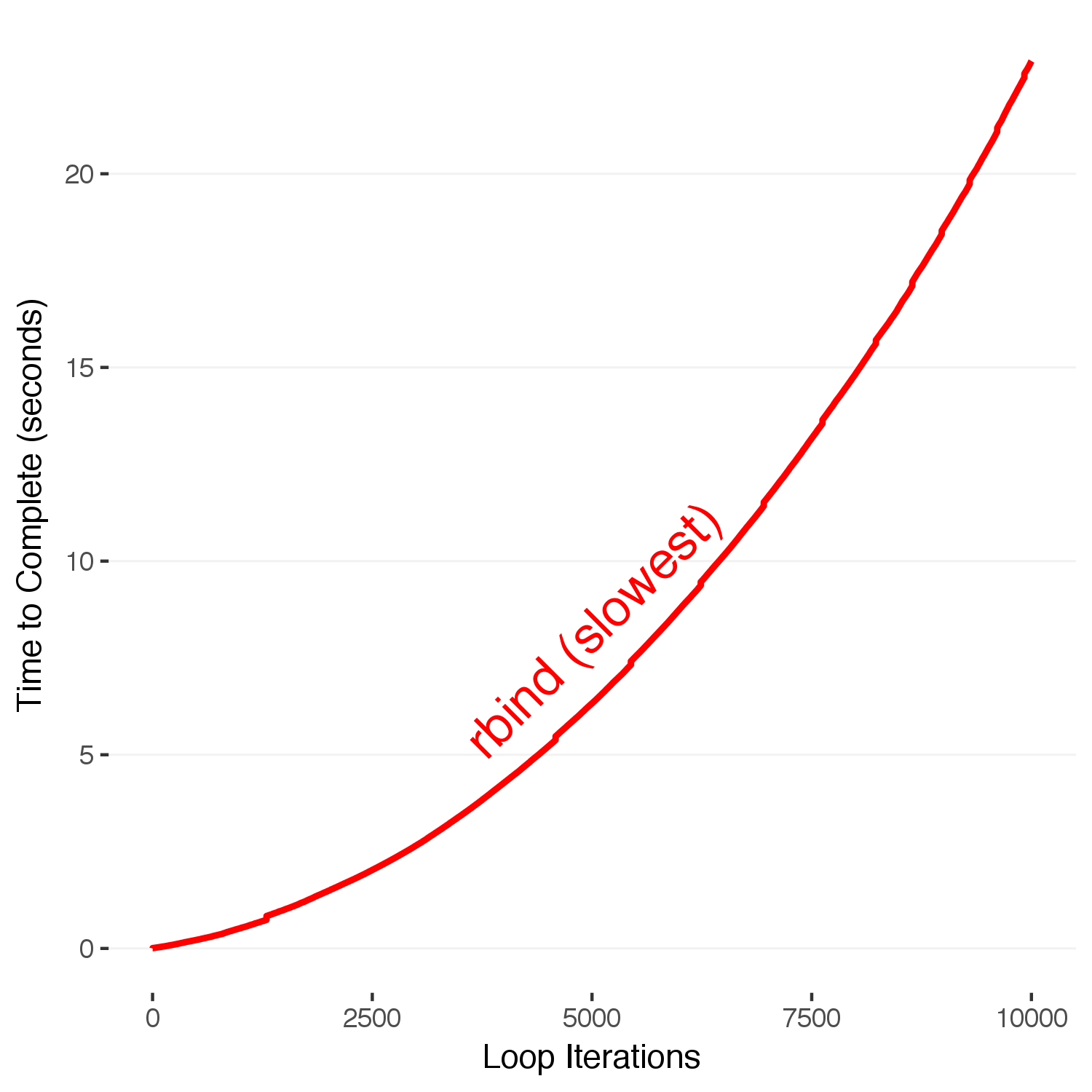
Here, we see that as the number of loops increases, the time required increases quadratically. This is because at each iteration \(N\) of the series, the total number of operations up to that point has been \(1+2+3+\dots +N\), which has an \(N^2\) dependence. To see this, we just have to count the number of operations R is doing under the hood for the entire loop, knowing that each iteration involves R copying the entire existing dataframe to add the one row on the end. Contrast that to the number of operations that one would expect if you were simply adding a row onto an existing dataframe without copying it.
generate_rect_coords = function(n) {
  counter = 1
  rects = list()
  for(i in 1:(n*(n+1)/2)) {
      rects[[counter]] = data.frame(xmin=-2,xmax=-1.5,ymin=i-1,ymax=i)
      counter = counter + 1
  }
  return(do.call(rbind,rects))
}

generate_point_coords = function(n) {
  counter = 1
  points = list()
  points[[counter]] = data.frame(x=0,y=0)
  counter = counter + 1
  for(i in 1:n) {
    points[[counter]] = data.frame(x=i,y=i*(i+1)/2)
    counter = counter + 1
  }
  return(do.call(rbind,points))
}

generate_rect_coords_linear = function(n) {
  counter = 1
  rects = list()
  for(i in 1:n) {
      rects[[counter]] = data.frame(xmin=-1,xmax=-0.5,ymin=i-1,ymax=i)
      counter = counter + 1
  }
  return(do.call(rbind,rects))
}

generate_point_coords_linear = function(n) {
  counter = 1
  points = list()
  points[[counter]] = data.frame(x=0,y=0)
  counter = counter + 1
  for(i in 1:n) {
    points[[counter]] = data.frame(x=i,y=i)
    counter = counter + 1
  }
  return(do.call(rbind,points))
}

ggplot() +
  geom_rect(data=generate_rect_coords(13),aes(xmin=xmin,xmax=xmax,ymin=ymin,ymax=ymax),fill="red",color="white") +
  geom_rect(data=generate_rect_coords(12),aes(xmin=xmin,xmax=xmax,ymin=ymin,ymax=ymax),fill="black",color="white") +
  geom_point(data=generate_point_coords(13),aes(x=x,y=y)) +
  geom_segment(data=data.frame(x=-0.5,xend=13,y=13*(13+1)/2,yend=13*(13+1)/2),aes(x=x,xend=xend,y=y,yend=yend),alpha=0.5,linetype="dashed",color="red") +
  scale_x_continuous(limits=c(-1,20)) +
  scale_y_continuous(limits=c(0,200)) +
  theme_tufte() +
  theme(text=element_text(family="Helvetica"),
        panel.grid.major.y = element_line(color = "grey95"))

ggplot() +
  geom_rect(data=generate_rect_coords(1),aes(xmin=xmin,xmax=xmax,ymin=ymin,ymax=ymax),fill="red",color="white",size=0.25) +
  geom_line(data=generate_point_coords(1),aes(x=x,y=y),size=0.5) +
  geom_rect(data=generate_rect_coords_linear(1),aes(xmin=xmin,xmax=xmax,ymin=ymin,ymax=ymax),fill="green",color="white",size=0.25) +
  geom_line(data=generate_point_coords_linear(1),aes(x=x,y=y),size=0.5) +
  scale_x_continuous("Loop Iteration", limits=c(-2,20)) +
  scale_y_continuous("Total Number of Memory Allocations",limits=c(0,150)) +
  theme_tufte() +
  theme(text=element_text(family="Helvetica"),
        panel.grid.major.y = element_line(color = "grey95"))
ggsave("iteration1.png",width=5,height=5,units="in",type="cairo")


for(size in 2:16) {
  ggplot() +
  geom_rect(data=generate_rect_coords(size),aes(xmin=xmin,xmax=xmax,ymin=ymin,ymax=ymax),fill="red",color="white",size=0.25) +
  geom_rect(data=generate_rect_coords(size-1),aes(xmin=xmin,xmax=xmax,ymin=ymin,ymax=ymax),fill="black",color="white",size=0.25) +
  geom_rect(data=generate_rect_coords_linear(size),aes(xmin=xmin,xmax=xmax,ymin=ymin,ymax=ymax),fill="green",color="white",size=0.25) +
  geom_rect(data=generate_rect_coords_linear(size-1),aes(xmin=xmin,xmax=xmax,ymin=ymin,ymax=ymax),fill="darkgreen",color="white",size=0.25) +
  geom_line(data=generate_point_coords_linear(size),aes(x=x,y=y),size=0.5,color="darkgreen") +
  geom_line(data=generate_point_coords(size),aes(x=x,y=y),size=0.5) +
  geom_segment(data=data.frame(x=-1.5,xend=size,y=size*(size+1)/2,yend=size*(size+1)/2),aes(x=x,xend=xend,y=y,yend=yend),alpha=0.5,linetype="dashed",color="red") +
  geom_segment(data=data.frame(x=-0.5,xend=size,y=size,yend=size),aes(x=x,xend=xend,y=y,yend=yend),alpha=0.5,linetype="dashed",color="green") +
  scale_x_continuous("Loop Iteration", limits=c(-2,20)) +
  scale_y_continuous("Total Number of Memory Allocations",limits=c(0,150)) +
  theme_tufte() +
  theme(text=element_text(family="Helvetica"),
        panel.grid.major.y = element_line(color = "grey95"))
  ggsave(paste0("iteration",size,".png"),width=5,height=5,units="in",type="cairo")
}

ggplot() +
  geom_rect(data=generate_rect_coords(size),aes(xmin=xmin,xmax=xmax,ymin=ymin,ymax=ymax),fill="red",color="white",size=0.25) +
  geom_rect(data=generate_rect_coords(size-1),aes(xmin=xmin,xmax=xmax,ymin=ymin,ymax=ymax),fill="black",color="white",size=0.25) +
  geom_rect(data=generate_rect_coords_linear(size),aes(xmin=xmin,xmax=xmax,ymin=ymin,ymax=ymax),fill="green",color="white",size=0.25) +
  geom_rect(data=generate_rect_coords_linear(size-1),aes(xmin=xmin,xmax=xmax,ymin=ymin,ymax=ymax),fill="darkgreen",color="white",size=0.25) +
  geom_line(data=generate_point_coords_linear(size),aes(x=x,y=y),size=0.5,color="darkgreen") +
  geom_line(data=generate_point_coords(size),aes(x=x,y=y),size=0.5) +
  geom_segment(data=data.frame(x=-1.5,xend=size,y=size*(size+1)/2,yend=size*(size+1)/2),aes(x=x,xend=xend,y=y,yend=yend),alpha=0.5,linetype="dashed",color="red") +
  geom_segment(data=data.frame(x=-0.5,xend=size,y=size,yend=size),aes(x=x,xend=xend,y=y,yend=yend),alpha=0.5,linetype="dashed",color="green") +
  annotate("text", label="O(n^2)",x=18,y=140,parse=TRUE,size=6) +
  annotate("text", label="O(n)",x=18,y=18,parse=TRUE,size=6) +
  scale_x_continuous("Loop Iteration", limits=c(-2,20)) +
  scale_y_continuous("Total Number of Memory Allocations",limits=c(0,150)) +
  theme_tufte() +
  theme(text=element_text(family="Helvetica"),
        panel.grid.major.y = element_line(color = "grey95"))
  ggsave(paste0("iteration",17,".png"),width=5,height=5,units="in",type="cairo")
We can see this is just the series:
\[1 + 2 + 3 + \dots + N\]
that can also be expressed in terms of the total number of loops, \(N\):
\[\sum^N_{i=1} i = \frac{N(N+1)}{2}\]
So how do you do this correctly? If you looked at the code above that I used to build the data to plot, you might notice that the functions I wrote to create the data use a list to store the results. This is because adding an entry to the end of a list does NOT copy the entire data structure during each loop. Thus, the time it takes to complete scales up linearly with the number of runs. Let’s time how long it takes to accumulate data with this method.
# Here, we initialize a list to store our output. Instead of appending a row to the end of a dataframe on each step, we append that row to the end of this list. Unlike the rbind method, this does NOT copy the entire existing dataframe with each iteration. Here is an odd R-ism: For an R list, to access the actual value stored inside the list you need to use double brackets [[1]] as opposed to a single bracket. For a fair comparison, we time the amount of time it takes to both put the list together (the inner loop) as well as combine it into the final dataframe with do.call(). For consistency with the previous method, I call proc.time in the interior loop even though its value isn't used.

finallist = list()

for(max in 1:10000) {
  initialtime = proc.time()[3]
  templist = list()

  for(i in 1:max) {
    templist[[i]] = data.frame(iteration = i, time = proc.time()[3] - initialtime)
  }
  temp = do.call(rbind,templist)

  finallist[[max]] = data.frame(iteration=max,time = proc.time()[3] - initialtime)
}

# Now we combine all of the dataframe rows in the list into one large dataframe, using the function do.call().

finalfast = do.call(rbind,finallist)

# What about nested loops? Use a counter variable and put it right below your list assignment. We can now nest to our hearts content with no performance loss.

initialtime = proc.time()[3]
finallist_2 = list()
counter = 1

for(i in 1:100) {
  for(j in 1:100) {
    finallist_2[[counter]] = data.frame(iteration = i, time = proc.time()[3]-initialtime)
    counter = counter + 1
  }
}

# If you need to record the iteration on each loop, assign the loop iterator as a property of the dataframe. Here, the $ operator is R shorthand for calling the column of that name. It's the same as if you typed in mydataframe["outerloop"] = i. We don't use this notation here because we are accessing the list with the [[counter]] index, and the resulting code block would look like finallist[[counter]]["outerloop"], which is, well, a lot of brackets. The final dataframe will have two extra columns (i,j) that correctly record the iteration information.

counter = 1
for(i in 1:100) {
  for(j in 1:100) {
    finallist_2[[counter]] = data.frame(iteration = i, time = proc.time()[3]-initialtime)
    finallist_2[[counter]]$outerloop = i
    finallist_2[[counter]]$innerloop = j
    counter = counter + 1
  }
}


# Plot the data.

ggplot() +
  geom_line(data=finalslow,aes(x=iteration,y=time),color="red",size=1) +
  geom_line(data=finalfast,aes(x=iteration,y=time),color="blue",size=1) +
  annotate("text",label="rbind (slowest)",x=5000,y=7.75,hjust=0.5,color="red",size = 4,angle=45) +
  annotate("text",label="list of rows (faster)",x=9000,y=3.5,hjust=1,color="blue",size = 4,angle=8) +
  scale_y_continuous("Time to Complete (seconds)") +
  scale_x_continuous("Loop Iterations") +
  theme_tufte() +
  theme(text=element_text(family="Helvetica"),
        panel.grid.major.y = element_line(color = "grey90"))

ggsave("rbindvslistrows.png",width=5,height=5,units="in",type="cairo")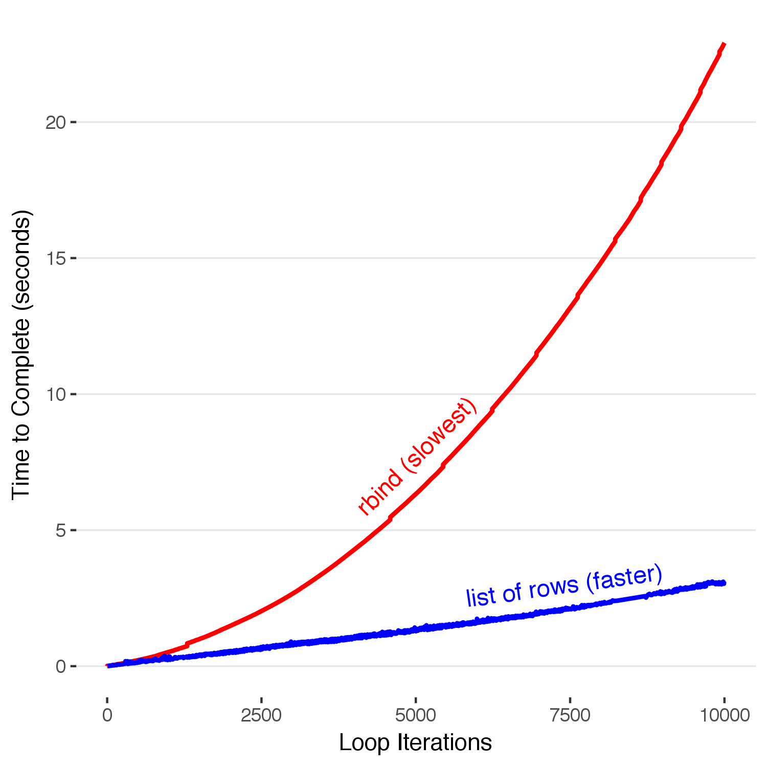
Here, we see that by appending to the end of a list and rbind-ing the whole dataframe together at the end the time it takes to build our completed dataframe only increases linearly with each iteration, a huge improvement. Stopping here and resting on our \(O(n)\) laurels, however, would hide the fact that this is still pretty slow. 10,000 iterations in 3 seconds means we have about 3,333 iterations per second. Building a million row dataframe with this method will take five minutes–which is enough time to make a cup of coffee, accidentally spill it all over yourself, and then have no one to blame but yourself for using an un-optimized data accumulation method. We must go faster.
Building a million row dataframe with this method will take five minutes–which is enough time to make a cup of coffee, accidentally spill it all over yourself, and then have no one to blame but yourself for using an un-optimized data accumulation method.
To speed up our loops, we need to know how R operates under the hood. R dataframes, as it turns out to be, aren’t ideal when accumulating data row by row. One of the reasons dataframes are slow is because they perform additional checks every time you add new data, such as type checking so that all of the entries for that column are the same class (factor, integer, numeric, character, boolean) and warning you when you add something that isn’t. When you are only passing in a single row, these checks aren’t necessary.
If speed is really your highest priority, you can forgo the niceties of dataframes and great deal of speed by accumulating your data in vectors within lists. This method barely increases code complexity, but provides a significant performance boost (5x). Here, we create a list to store our data, exactly like we did in the previous step. Rather than filling each list entry with a row of a dataframe, however, we are creating a list with two entries, each containing a plain R vector to which we add our data. This is still able to be transformed into a dataframe with do.call() because dataframes are just structured as a collection of lists shown as columns.
faster_final = list()

for(max in 1:10000) {
  templist = list(iteration=0, time=0)
  initialtime = proc.time()[3]

  for(i in 1:max) {
    templist$iteration[i] = i
    templist$time[i] = proc.time()[3] - initialtime
  }
  temp = do.call(rbind,templist)

  faster_final[[max]] = data.frame(iteration=max,time = proc.time()[3] - initialtime)
}

fastest = do.call(rbind,faster_final)


ggplot() +
  geom_line(data=finalslow,aes(x=iteration,y=time),color="red",size=1) +
  geom_line(data=finalfast,aes(x=iteration,y=time),color="blue",size=1) +
  geom_line(data=fastest,aes(x=iteration,y=time),color="green",size=1) +
  annotate("text",label="rbind (slowest)",x=1200,y=2.5,hjust=0.5,color="red",size = 4,angle=0) +
  annotate("text",label="list of rows (faster)",x=9000,y=3.4,hjust=1,color="blue",size = 4,angle=8) +
  annotate("text",label="list of vectors (even faster)",x=10000,y=1.30,hjust=1,color="green",size = 4,angle=3) +
  theme_tufte() +
  scale_y_continuous("Time to Complete (seconds)") +
  scale_x_continuous("Loop Iterations") +
  theme(text=element_text(family="Helvetica"),
        panel.grid.major.y = element_line(color = "grey90"))

ggsave("rbindvslistvsvectors.png",width=5,height=5,units="in",type="cairo")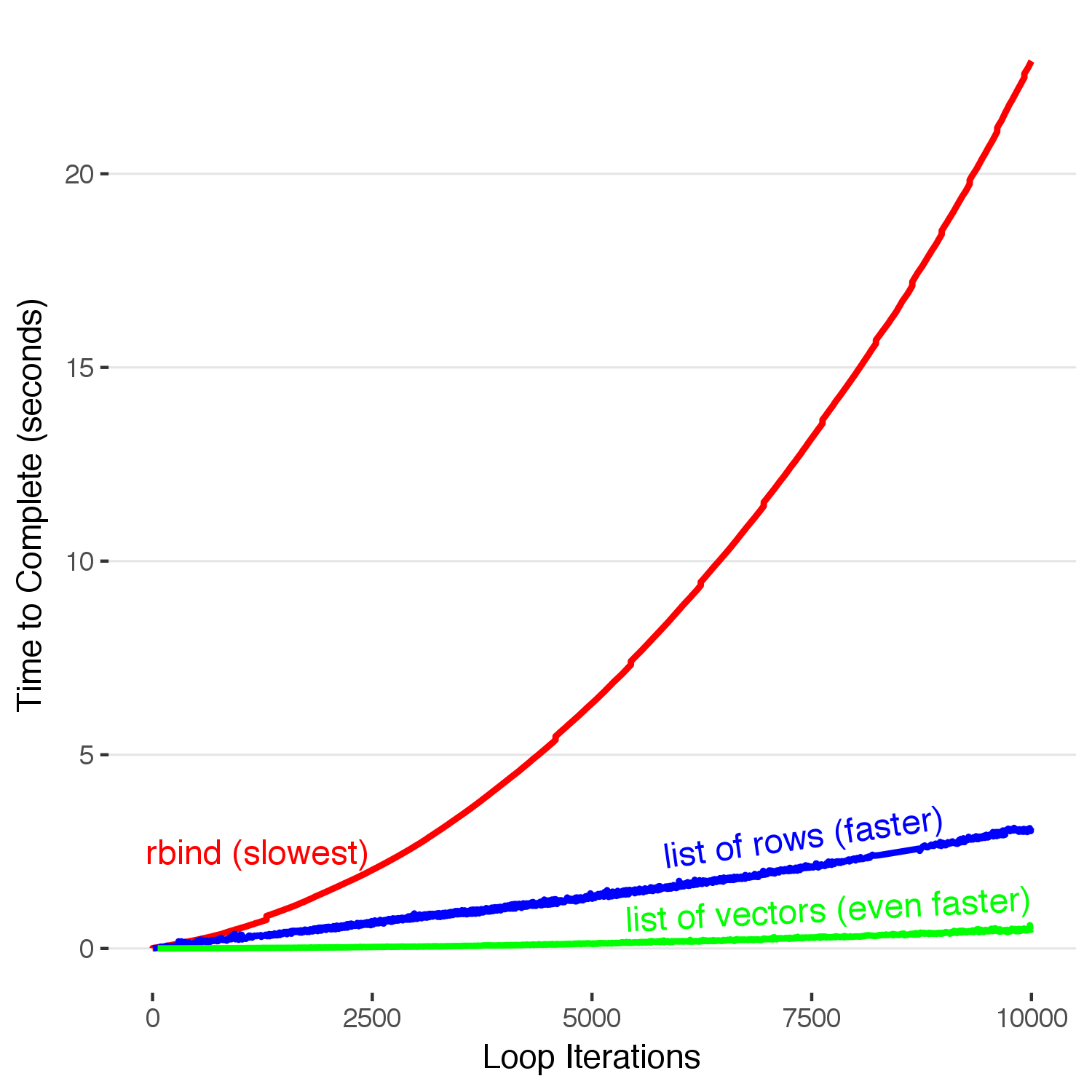
Much faster, and with hardly any increase in complexity. Notice how we still use the do.call(rbind, … ) idiom. Now accumulating our 1 million row dataframe will only take 1 minute, a significant improvement. However, 1 minute of free time is short enough that you can’t do anything else while you wait, but long enough to stare at the your screen and let your mind wander to unproductive places.
We must go faster. We can do this by pre-allocating our vectors before we accumulate into them.
fastest_final = list()

for(max in 1:10000) {

  initialtime = proc.time()[3]
  templist = list()
  templist$iteration = rep(0,10000) #pre-allocating 10,000 slots
  templist$time = rep(0,10000)      #pre-allocating 10,000 slots

  for(i in 1:max) {
    templist$iteration[i] = i
    templist$time[i] = proc.time()[3] - initialtime
  }

  temp = do.call(rbind,templist)

  fastest_final[[max]] = data.frame(iteration=max,time = proc.time()[3] - initialtime)
}

fastestest = do.call(rbind,fastest_final)


ggplot() +
  geom_line(data=finalslow,aes(x=iteration,y=time),color="red",size=0.5) +
  geom_line(data=finalfast,aes(x=iteration,y=time),color="blue",size=0.5) +
  geom_line(data=fastest,aes(x=iteration,y=time),color="green",size=0.5) +
  geom_line(data=fastestest,aes(x=iteration,y=time),color="darkgreen",size=0.5) +
  annotate("text",label="rbind (don't bother)",x=3200,y=3.2,hjust=1,color="red",size = 2,angle=75) +
  annotate("text",label="list of rows (faster)",x=7500,y=2.35,hjust=1,color="blue",size = 3,angle=40) +
  annotate("text",label="list of vectors (even faster)",x=9700,y=0.6,hjust=1,color="green",size = 3,angle=12) +
  annotate("text",label="preallocated list of vectors (fastest)",x=9900,y=0.1375,hjust=1,color="darkgreen",size = 3,angle=1) +
  theme_tufte() +
  scale_y_continuous(limits=c(-0.1,3.3),"Time to Complete (seconds)") +
  scale_x_continuous("Loop Iterations",expand=c(0,0)) +
  theme(text=element_text(family="Helvetica"),
        panel.grid.major.y = element_line(color = "grey90"))

ggsave("preallocationvseverything.png",width=5,height=5,units="in",type="cairo")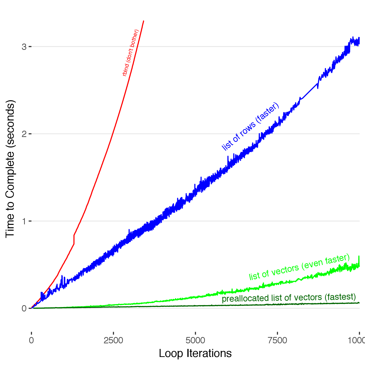
Pre-allocating our vectors within our list results in the best performance, by far. We see here a 10x speed up compared to not preallocating, which itself was a 5x improvement over adding to our list of dataframe rows, which itself was massive increase in performance over the naive method of rbind-ing rows onto a dataframe. Note that you can also see how the unpreallocated vector curves up, showing a slight \(O(n^2)\) dependence. When you add a new entry to the end of a vector, it does in fact copy the whole vector each iteration. Thus, the time will grow as \(O(n^2)\) (but not as badly as the first case). Our 1 million row dataframe now takes 6 seconds to build, hardly enough time to consider deep existential threats to the universe. With the proper tools now at our disposal, we can now write fast and efficient R code.
One downside of pre-allocating memory arises when you’re running a dynamic loop with an unknown duration and you exceed your preallocated memory. What happens when you overflow this amount? Below, I simulate the same process as above, except now we have only pre-allocated half of the required memory.
half_allocate = list()

for(max in 1:10000) {
  initialtime = proc.time()[3]
  templist = list()
  templist$iteration = rep(0,5000)
  templist$time = rep(0.0,5000)

  for(i in 1:max) {
    templist$iteration[i] = i
    templist$time[i] = proc.time()[3] - initialtime
  }

  temp = do.call(rbind,templist)

  half_allocate[[max]] = data.frame(iteration=max,time = proc.time()[3] - initialtime)
}

half_allocate_df = do.call(rbind,half_allocate)


ggplot() +
  geom_line(data=newfastest,aes(x=iteration,y=time),color="red",size=0.5) +
  geom_line(data=newfastestest,aes(x=iteration,y=time),color="green",size=0.5) +
  geom_line(data=half_allocate_df,aes(x=iteration,y=time),color="orange",size=0.5) +
  geom_segment(aes(x=5000,xend=5000,y=0,yend=0.6),linetype="dashed",color="red",alpha=0.3,size=0.5) +
  annotate("text",label="Zero Pre-allocated",x=3000,y=0.1,hjust=1,color="red",size = 4,angle=0) +
  annotate("text",label="Half Pre-allocated",x=10000,y=0.095,hjust=1,color="orange",size = 4,angle=0) +
  annotate("text",label="All Pre-allocated",x=10000,y=0.02,hjust=1,color="green",size = 4,angle=0) +
  theme_tufte() +
  scale_y_continuous(limits=c(-0.01,0.6),"Time to Complete (seconds)") +
  scale_x_continuous(limits=c(0,10000),"Loop Iterations") +
  theme(text=element_text(family="Helvetica"),
        panel.grid.major.y = element_line(color = "grey90"))

ggsave("halfpreallocation.png",width=5,height=5,units="in",type="cairo")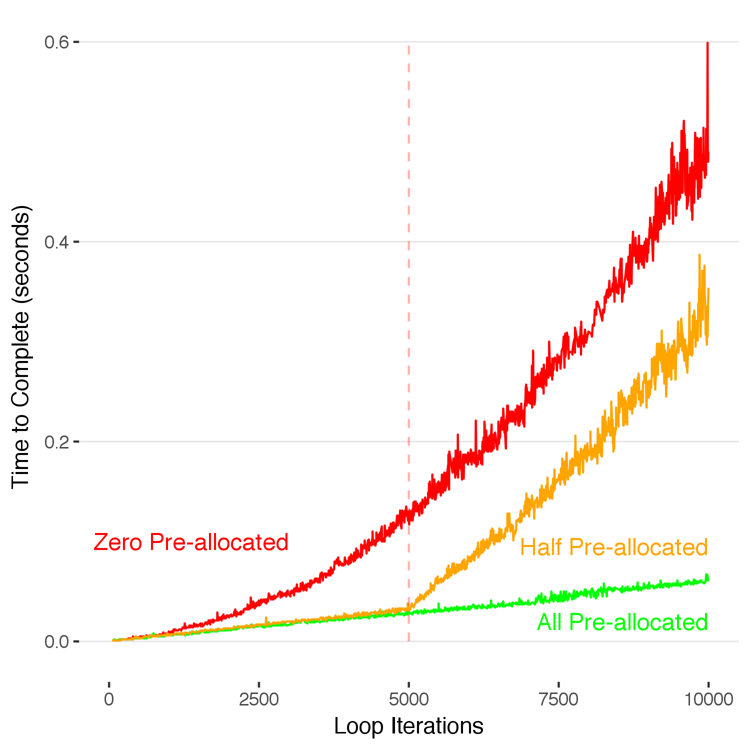
Once we exceed our original preallocated 5,000 slots, R allocates new memory on the fly and thus the time-to-complete starts increasing from that point at the same rate as in the unallocated case. An efficient way to fix this problem would be to copy the completed 5,000 data points into a new data structure with 10,000 spots when it fills up, and then we would only have to reallocate new memory once per 5,000 runs, rather than at the end of each run. This is a flexible middle ground between the two approaches.
If you carefully looked at the code I used to generate these figures you might have noticed that throughout, I use the slower of the \(O(n)\) methods: rbind-ing a list of dataframe rows together. Due to the complexity of many R calculations, it will be rare that the method used to accumulate data will be the weakest link in the time it takes to complete an R script. Thus, using a method with a low mental overhead and robust type-checking and other niceties is usually worth the lost efficiency. Premature optimization is the root of all evil. However, when you are running large simulations that involve accumulating large amounts of data and possibly paying for server time, you now have the tools to ensure that you are using the most efficient methods available.
Now, finally, we return to the original statement: can you forgo the apply family of functions and use for loops entirely? We now know how to properly record data when using for loops, but when we do repeated operations on a matrix does using a loop introduce any penalty over apply()? Let’s find out.
testapply = list()

# First, we generate a 10001 x 10001 matrix of random numbers pulled from a gaussian distribution. Our goal is to sum each of the columns and return a vector of each sum. Here, we have two strategies:

# 1) Loop through each column, calculate the sum, and assign into a vector.
# 2) apply() the sum function to each column.

numbers = matrix(rnorm(10001^2,0,1),nrow=10001,ncol=10001)
iter=1

for(max in seq(1,10001,25)) {

  nnumbers = numbers[,1:max,drop=FALSE]

  # Calling gc() (which tells R to clean up memory) consistently before each run will make timing the operations much more consistent. Without this call, the timing results are noisy.

  gc()

  # First: the for loop.

  initialtime = proc.time()[3]
  totalsum = rep(0,max)
  for(i in 1:max) {
    totalsum[i] = sum(nnumbers[,i,drop=FALSE]))
  }
  testapply$timeloop[iter] = proc.time()[3] - initialtime

  # Now timing the apply function. The 2 in apply() tells R to sum the matrix nnumbers by column.

  initialtime = proc.time()[1]
  totalsum = apply(nnumbers,2,sum)
  testapply$timeapply[iter] = proc.time()[3] - initialtime

  testapply$iteration[iter] = max
  iter = iter + 1
}

forvsapplydf = do.call(cbind,testapply)


forvsapplydf %>%
  ggplot() +
  geom_line(aes(x=iteration,y=timeloop),color="green") +
  geom_line(aes(x=iteration,y=timeapply),color="red") +
  scale_y_continuous(limits=c(-0.01,2),"Time to Complete (seconds)") +
  scale_x_continuous(limits=c(0,10001),"Matrix Size (10000 x N)") +
  annotate("text",label="apply()",x=8000,y=1.8,hjust=1,color="red",size = 6,angle=0) +
  annotate("text",label="for loop",x=8000,y=0.25,hjust=1,color="green",size = 6,angle=0) +
  annotate("text",label="gc()",x=2000,y=1.75,hjust=1,color="black",size = 6,angle=0) +
  theme_tufte() +
  theme(text=element_text(family="Helvetica"),
        panel.grid.major.y = element_line(color = "grey90"))

ggsave("applyvsforloopgc.png",width=5,height=5,units="in",type="cairo")
An animation that showing the difference between timing with and without manually calling gc(). 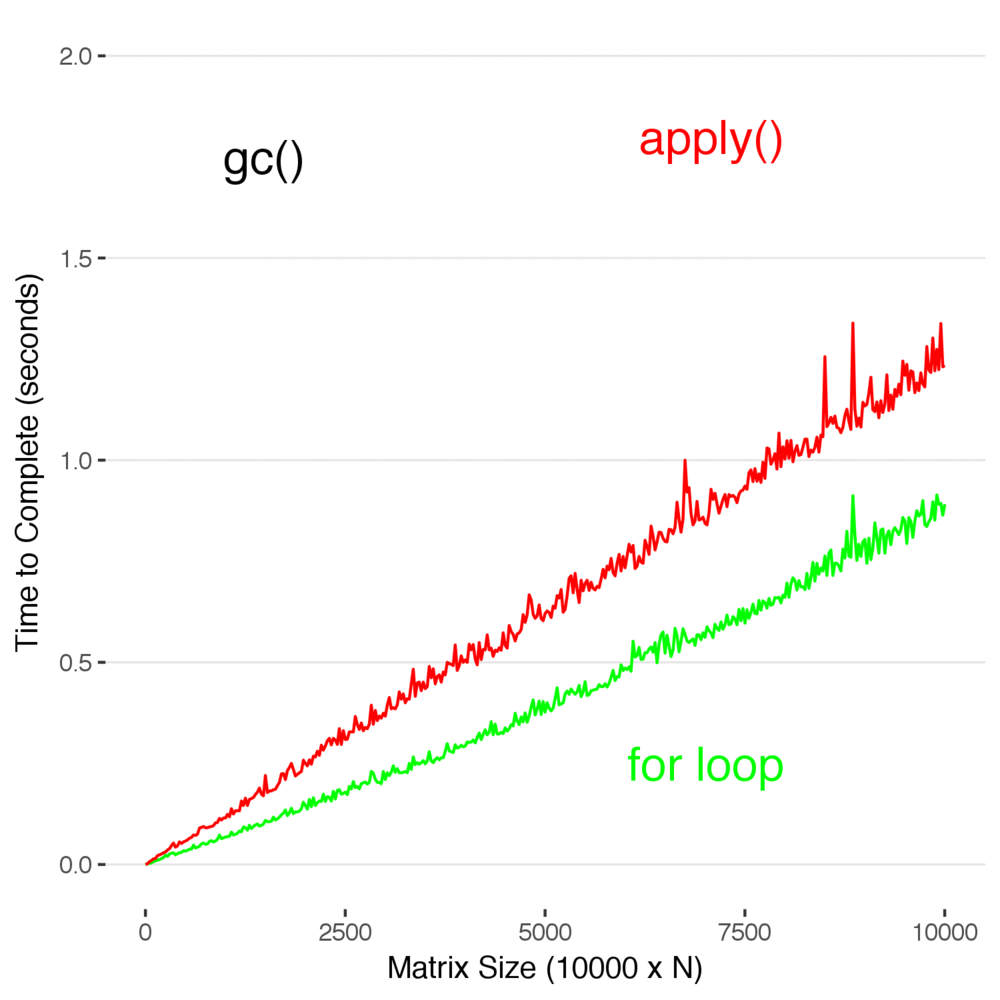
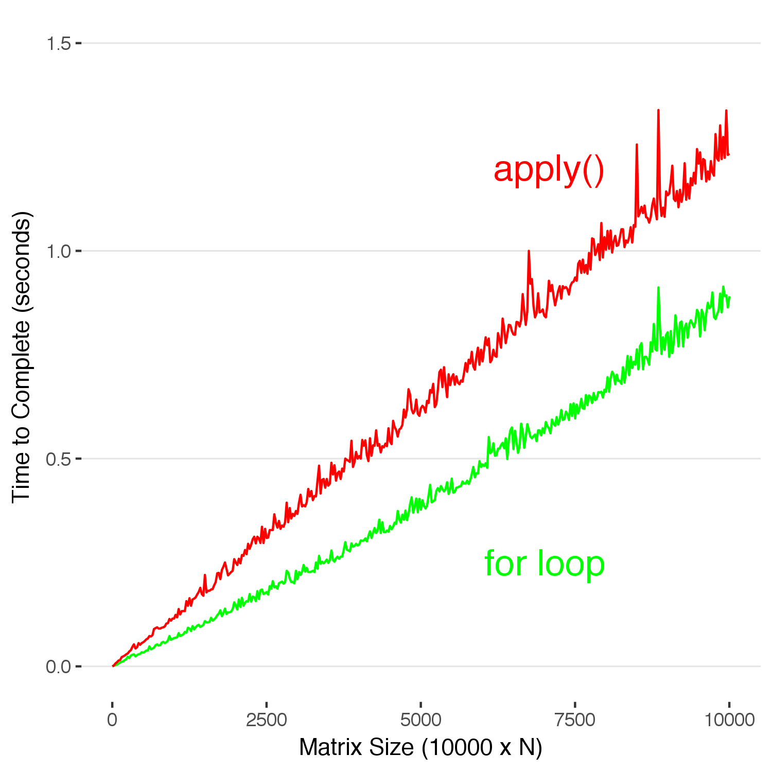
Look at that. In this case, using apply() is actually slower than using a for loop. Don’t read too deeply into this and decide this means you should stop using apply() , but you don’t have to use it to efficiently code in R. It’s not as elegant, but sometimes it’s just faster and easier to write a loop to manipulate data–and there is no real penalty for it..
Summary: We covered one of the main issues that has lead to R’s less-than-stellar reputation–slow speed–and have shown how it isn’t an issue at all. If you have prior experience programming, it should be easy to translate those programming idioms into this powerful analytical language.