Sculpting the Moon in R: Subdivision Surfaces and Displacement Mapping

Data Visualization

Mesh Processing

Rayshader

Rayrender

Rayvertex

Rayimage

Package Development

Displacement Mapping

Author

Tyler Morgan-Wall

We like the moon
The moon is very useful, everyone
Everybody like the moon
Because it light up the sky at night
and it lovely and it makes the tides go
and we like it
But not as much as cheese
We really like cheese

— The Spongmonkies, 2002

Introduction

TL;DR

In this post, we explore subdivision surfaces and displacement mapping within the rayverse, using the rayvertex, rayimage, and rayrender packages. We demonstrate how to create detailed and smooth 3D models by subdividing meshes and applying displacement textures. These techniques enhance both artistic and data visualization projects by providing realistic and intricate surface details.

Bumpy objects and smooth objects. These are the two demons you must slay if you want to be successful in 3D rendering.

Just kidding! There are thousands of demons you must slay. The princess is always in another castle.

Triangles, the primary building blocks of computer graphics, don’t directly lend themselves to either extremely smooth or realistically bumpy objects. Since triangles are flat primitives, borders between non-coplanar adjacent triangles will always have sharp edges. You can introduce approximations to work around this (such as per-vertex normals), but approximations always have failure modes, particularly with certain rendering algorithms. Bumpy objects suffer from the same issue: approximating a rough surface using a bump map or a normal map (which change the underlying surface normal without actually changing the geometry) can lead to non-physically accurate results.

There’s also NURBS, quadratic surfaces, curves, and more exotic objects

Historically, renderers worked around this by subdividing meshes into “micropolygons”: polygons smaller than a single pixel. This means triangle edges were not visible, as they only existed a on sub-pixel scale. This subdivision enabled the rendering of smooth objects and the rendered image no longer had visible discontinuities in the surface normal due to geometry. This subdivision process allowed for bumpy surfaces as well: by displacing the vertices of these micropolygons, you could easily generate highly detailed surfaces given a basic low-resolution mesh and a displacement texture. It can be significantly easier to work with displacement information in 2D form and use it to displace a low-resolution 3D mesh, rather than try to construct a fully-detailed 3D mesh directly.

The Reyes rendering algorithm–which brought us Toy Story and Star Trek II: Wrath of Khan–actually works off of quadrilaterals, not triangles, but the idea is the sameRayshader has always performed a basic version of displacement mapping when generating meshes, but it’s been limited to displacing a flat surface.

This brings us to why I implemented subdivision surfaces and displacement mapping in the rayverse: there’s plenty of 2D data out there and not all of it lives on a flat, Cartesian plane. If you’re plotting data that spans the entire planet (or moon!), there’s always a struggle to pick the right projection, knowing that there’s no ideal way to transform a sphere to 2D without warping the data in some way. Expressing the data in its native curved space avoids those issues entirely.

While 3D plotting has its own set of issues, it also has many advantages–see this blog post for more information

So let’s dive into subdivision surfaces and displacement mapping! What is it, how it was implemented, things to keep in mind when using it, and what you can do with it in the rayverse.

Subdivision

We’ll start by loading three useful rayverse packages: rayvertex to construct raymesh objects and manipulate them directly, rayimage to manipulate displacement textures and load a variety of image files, and rayrender to visualize these meshes in a high-quality pathtracer.

library(rayvertex)
library(rayimage)
library(rayrender)

Now, let’s render an image of some shapes with Loop subdivision. We’ll be using rayvertex because it renders faster and has more fine-grained control over the meshing process. Note here the new (as of rayvertex v0.11.0) print output showing a command-line preview of the materials, as well as a preview of the scene information.

Fun fact: Loop subdivision is not named after some cyclical mesh property or iterative process that the name might suggest: it’s actually named after the graphics researcher Charles Loop.

base_material = material_list(diffuse="red", ambient = "red",
                              type = "phong", shininess = 5,
                              diffuse_intensity = 0.8, ambient_intensity = 0.2)
base_material

1: Create and print the red cube material

• rayvertex_material
• type: phong
• diffuse: #ff0000   | intensity: 0.8
• ambient: #ff0000   | intensity: 0.2
• shininess: 5

base_material2 = material_list(diffuse="purple", ambient = "purple",
                               type = "phong", shininess = 5,
                               diffuse_intensity = 0.8, ambient_intensity = 0.2)
base_material2

1: Create and print the purple sphere material

• rayvertex_material
• type: phong
• diffuse: #a020f0   | intensity: 0.8
• ambient: #a020f0   | intensity: 0.2
• shininess: 5

Note how the materials print a preview of the actual colors and relevant (i.e. non-default) material settings. This is due to rayvertex’s new integration with the cli package and a whole collection of new pretty-print functions.

scene = cube_mesh(material = base_material, scale = 0.8) |>
  add_shape(sphere_mesh(radius=0.5,position = c(-1.2,0,0), low_poly = TRUE,
                        normals = TRUE,
                        material = base_material2)) |>
  add_shape(obj_mesh(r_obj(), position=c(1.2,0,0)))
scene

1: Create the 3D scene
2: Print the scene information

── Scene Description ───────────────────────────────────────────────────────────

• Summary - Meshes: 3 | Unique Materials: 4
ℹ XYZ Bounds - Min: c(-1.69, -0.51, -0.49) | Max: c(1.70, 0.49, 0.51)
             shapes  vertices texcoords   normals materials
          <ray_shp> <ray_dat> <ray_dat> <ray_dat> <ray_mat>
1   <T:12|UV|N|M:1>     <8x3>     <4x2>     <6x3>   <phong>
2   <T:48|UV|N|M:1>    <26x3>    <34x2>    <26x3>   <phong>
3 <T:2280|UV|N|M:6>  <1520x3>  <1520x2>    <none>      <6x>

The rayvertex scene information now also includes a dense, readable tabular summary of each individual mesh that makes up the scene. Rather than looking at a verbose print-out of lists of vertex data and material information, now you can get a sense of the scene at a glance.

rasterize_scene(scene, lookfrom = c(-4,3,10), lookat=c(-0.05,0,0),
                fov=9, height = 550, width=1100,
                light_info = directional_light(c(1,1,2)))

1: Render the scene

We’ve now rendered some basic low-polygon shapes. Low-polygon here means that you can clearly see lighting artifacts from the chunky triangles that make up the mesh: there are discontinuities on the sphere from the vertex normal interpolation, resulting in unphysical “lines” of light that run along the edges of the triangles.

Let’s subdivide the meshes with the new subdivide_mesh() function and determine how many subdivisions renders any individual triangle too small to see. Each subdivision level increases the number of triangles by a factor of four. We won’t initially add vertex normals so we can see exactly what’s going on with the geometry.

scene |> 
  subdivide_mesh(subdivision_levels = 2, normals = FALSE) |>
  rasterize_scene(lookfrom = c(-4,3,10), lookat=c(-0.05,0,0),
                  fov=9, height = 550, width=1100,
                  light_info = directional_light(c(0.2,1,2)))

1: Subdivide the scene

Note how the cube has shrunk considerably and the sharp edges of the letter R have collapsed in on themselves. This phenomenon occurs because subdivision algorithms, like Loop subdivision, work by averaging the positions of vertices to create a smoother surface. Sharp edges consisting of large triangles will be much more affected by this process. To fix this, we can turn off vertex interpolation and first apply a non-interpolated simple subdivision step and then follow it up with regular Loop subdivision step to more accurately maintain the initial shape of the object.

scene |> 
  subdivide_mesh(normals = FALSE, simple = TRUE) |>
  subdivide_mesh(subdivision_levels = 2, normals = FALSE) |>
  rasterize_scene(lookfrom = c(-4,3,10), lookat=c(-0.05,0,0),
                  fov=9, height = 550, width=1100,
                  light_info = directional_light(c(0.2,1,2)))

1: Subdivide the scene but don’t smooth the mesh
2: Subdivide the scene normally, but don’t calculate normals to better show the triangle faces

Note how the cube is still cube-ish, but with nicely curved edges! The R logo looks nicer here too, as the large corner that makes up the R didn’t collapse. The only problem is the low-poly sphere is now more like a 20-sided D&D die, which isn’t great if you’d like the limit of the subdivision process to result in an identical (but smoothed) version of the original mesh. But it’s nice to have a workflow for adding rounded bevels to models, which adding a simple subdivision step provides. Let’s get back to trying to trying to subdivide until we can’t tell the mesh is made of individual triangles anymore. How about three subdivisions?

scene |> 
  subdivide_mesh(subdivision_levels = 3, normals = FALSE) |>
  rasterize_scene(lookfrom = c(-4,3,10), lookat=c(-0.05,0,0),
                  fov=9, height = 550, width=1100,
                  light_info = directional_light(c(0.2,1,2)))

1: Subdivide the objects three times

Not yet. Still visible. Let’s subdivide again.

scene |> 
  subdivide_mesh(subdivision_levels = 4, normals = FALSE) |>
  rasterize_scene(lookfrom = c(-4,3,10), lookat=c(-0.05,0,0),
                  fov=9, height = 550, width=1100,
                  light_info = directional_light(c(0.2,1,2)))

1: Subdivide the objects four times

Almost! But no cigar.

scene |>
  subdivide_mesh(subdivision_levels = 5, normals = FALSE) ->
scene_5x

rasterize_scene(scene_5x, lookfrom = c(-4,3,10), lookat=c(-0.05,0,0),
                fov=9, height = 550, width=1100,
                light_info = directional_light(c(0.2,1,2)))

1: Render the scene
2: Subdivide the mesh five times and save it to an object

There we go. We can compare the before and after mesh sizes to see how mary more triangles this required to reach continuity. Note the number of vertices and the T: field in the shapes column indicating the number of triangles.

print(scene)

1: Printing the scene information before subdivision

── Scene Description ───────────────────────────────────────────────────────────

• Summary - Meshes: 3 | Unique Materials: 4
ℹ XYZ Bounds - Min: c(-1.69, -0.51, -0.49) | Max: c(1.70, 0.49, 0.51)
             shapes  vertices texcoords   normals materials
          <ray_shp> <ray_dat> <ray_dat> <ray_dat> <ray_mat>
1   <T:12|UV|N|M:1>     <8x3>     <4x2>     <6x3>   <phong>
2   <T:48|UV|N|M:1>    <26x3>    <34x2>    <26x3>   <phong>
3 <T:2280|UV|N|M:6>  <1520x3>  <1520x2>    <none>      <6x>

print(scene_5x)

1: Printing the scene information after subdivision

── Scene Description ───────────────────────────────────────────────────────────

• Summary - Meshes: 3 | Unique Materials: 4
ℹ XYZ Bounds - Min: c(-1.63, -0.45, -0.45) | Max: c(1.70, 0.46, 0.45)
                shapes    vertices   texcoords   normals materials
             <ray_shp>   <ray_dat>   <ray_dat> <ray_dat> <ray_mat>
1   <T:12288|UV|N|M:1>    <6146x3>    <6146x2>    <none>   <phong>
2   <T:49152|UV|N|M:1>   <24578x3>   <24578x2>    <none>   <phong>
3 <T:2334720|UV|N|M:6> <1167360x3> <1167360x2>    <none>      <6x>

Yikes! We can see it grew by a lot: Five subdivision levels resulted in a \(4^5 = 1024\)x increase in the mesh size. Of course, we can turn the normals option back on, which then calculates smoothed vertex normals. With vertex normals, we only need three subdivision levels to achieve the same visual fidelity as the 5x subdivided mesh. Since the triangles are relatively small compared to the low-poly original, we won’t see the same sort of lighting discontinuities noted in the first render.

translate_mesh(subdivide_mesh(scene, subdivision_levels = 3) ,position=c(0,1.1,0)) |> 
  add_shape(scene_5x) |> 
  add_shape(translate_mesh(scene,position=c(0,2.2,0))) |> 
  rasterize_scene(lookfrom = c(-4,3,10), lookat=c(-0.05,1.1,0),
                  fov=18, height = 1100, width=1100,
                  light_info = directional_light(c(0.2,1,2)))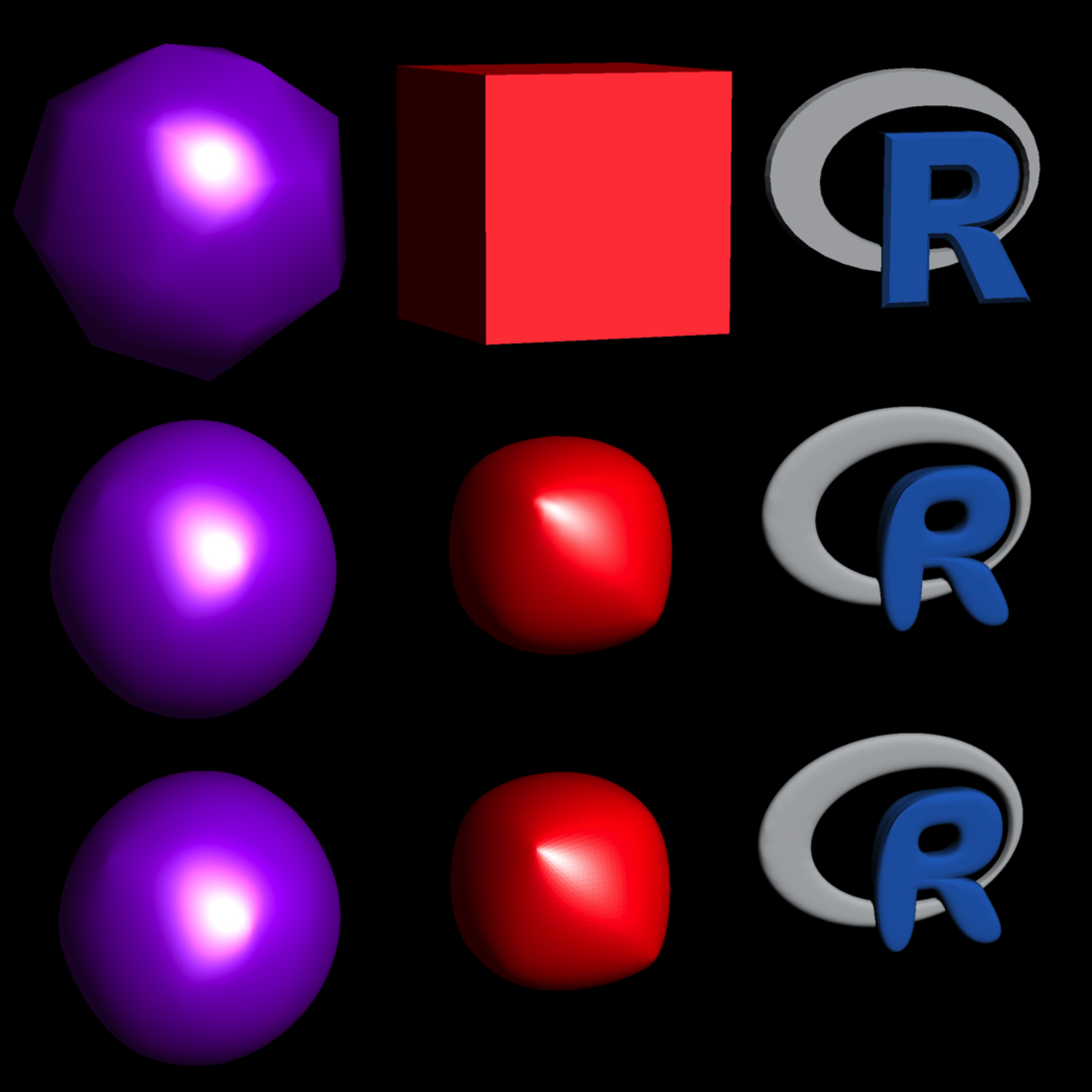

Figure 1: Top Row: Original low-poly meshes. Middle Row: Highly subdivided (1024x triangles) scene without vertex normals. Bottom Row: 3x subdivided scene (64x triangles) with vertex normals.

And that’s it for subdivision surfaces, at least for now!

Displacement Mapping

We just subdivided a low-red mesh to make it smooth–how do we make it bumpy? We can do that by applying a displacement texture, which offsets each vertex via its vertex normal. Here’s an example of a displacement texture of the moon:

If there aren’t any vertex normals in the mesh, it first calculates them by averaging the directions of all the faces connected to a single vertex. This interface also supports vector displacement, but I’m not going to get into that in this post

disp_moon = ray_read_image("../images/2024/ldem_3_8bit.jpg") 
plot_image(disp_moon)

Higher regions are lighter, and depressions are darker. If you’ve used worked in GIS software or with rayshader before, you might ask: isn’t this just a digital elevation model (DEM)? Sure is! Let’s check out the Monterey Bay data included in rayshader to see:

library(rayshader) 

montereybay |>
  height_shade(texture = colorRampPalette(c("black","white"))(100)) |>
  plot_map()

1: Use rayshader to plot the black to white color mapping of the Monterey Bay DEM

What displacement mapping does is allow this type of transformation to be applied to any 3D surface, rather than just a 2D plane (as in rayshader). So displacement mapping allows us to apply these displacements to a sphere. In a universe full of spheres and ellipsoids, this capability can be quite useful. Our image data ranges from 0-1 in this case, and the difference (from the mean elevation) between the highest point on the moon (6.7 miles) and the lowest (-5.4 miles) is 12.1 miles, which when compared to the moon’s radius (1,079.6 miles) is about a 1.1 percent variation. So with a unit sphere representing the moon, our displacement scale is 0.011.

Let’s visualize the displacement on a basic small sphere mesh. :

I have to call smooth_normals_mesh() and add_sphere_uv_mesh() because the displacement algorithm here requires one UV coordinate/normal per vertex

lights = directional_light(c(1,0,0)) |>
  add_light(directional_light(c(-1,0,0),
                              color="dodgerblue",
                              intensity=1))

white_material = material_list(diffuse = "white",
                               ambient = "white",
                               diffuse_intensity = 0.9,
                               ambient_intensity = 0.1)

sphere_mesh(material = white_material) |>
  smooth_normals_mesh() |>
  add_sphere_uv_mesh(override_existing = TRUE) ->
basic_sphere_uv

basic_sphere_uv |>
  displace_mesh(disp_moon, displacement_scale = 0.011) |>
  rasterize_scene(light_info = lights, width = 1100, height = 550, fov=13)

1: Generate the lighting for the scene
2: Generate the basic white material for the sphere
3: Create a smooth sphere and add unique normals and UV coordinates for each vertex
4: Displace the sphere with the moon data, scaled by 0.011, and render it

Displacing mesh with 512x1024 texture

Setting `lookat` to: c(-0.00, -0.00, 0.00)

Wait–nothing happened? What went wrong? Well, let’s look at the mesh info and compare the number of vertices in the mesh to the resolution of the image:

basic_sphere_uv

── Scene Description ───────────────────────────────────────────────────────────

• Summary - Meshes: 1 | Unique Materials: 1
ℹ XYZ Bounds - Min: c(-1.00, -1.00, -1.00) | Max: c(1.00, 1.00, 1.00)
            shapes  vertices texcoords   normals materials
         <ray_shp> <ray_dat> <ray_dat> <ray_dat> <ray_mat>
1 <T:960|UV|N|M:1>   <482x3>   <482x2>   <482x3> <diffuse>

dim(disp_moon)
prod(dim(disp_moon)[1:2])

1: Multiply the dimensions of the texture together to get the number of pixels

[1]  512 1024    3
[1] 524288

So there’s half a million points, but only about 500 total vertices. Let’s write a function to show ourselves exactly where and how much of the displacement map we’re sampling. The green pixels are the places in the elevation model we are actually using to displace out mesh.

get_displacement_access_info = function(mesh, image) {
  image_coords = round(matrix(dim(image)[2:1]-1,ncol=2,
                         nrow=nrow(mesh$texcoords[[1]]),
                         byrow=TRUE) * mesh$texcoords[[1]])

  for(i in seq_len(nrow(image_coords))) {
    image[1+image_coords[i,2],1+image_coords[i,1],1:3] = c(0,1,0)
  }
  total_pixels = as.integer(prod(dim(image)[1:2]))
  total_pixels_sampled = as.integer(sum(image[,,1] == 0 & image[,,2] == 1 & image[,,3] == 0))
  message(sprintf("Total pixels sampled: %i/%i (%0.5f%%)",
                  total_pixels_sampled, total_pixels, total_pixels_sampled/total_pixels*100))
  plot_image(image)
}
get_displacement_access_info(basic_sphere_uv, disp_moon )

1: Take the UV coordinates (which range from 0-1) and map them to the pixel coordinates by multiplying the number of rows and columns by each UV pair.
2: Loop over the image and set each accessed pixel to green.
3: Calculate the total number of pixels.
4: Calculate the total number of accessed (green) pixels.
5: Print the access information.
6: Plot the image with green pixels marking data used to displace the mesh.

Total pixels sampled: 482/524288 (0.09193%)

So, we’re sampling 0.092% of the pixels in the image–no wonder it’s such a poor approximation! Let’s use subdivision to increase the size of our mesh, which should sample more of the underlying displacement texture and thus give us a better approximation.

generate_moon_mesh = function(subdivision_levels, displacement_texture, displacement_scale) {
  sphere_mesh(material = white_material) |> 
    smooth_normals_mesh() |> 
    subdivide_mesh(subdivision_levels = subdivision_levels) |>
    add_sphere_uv_mesh(override_existing = TRUE) |>
    displace_mesh(displacement_texture, displacement_scale) |>
    rotate_mesh(c(0,90,0))
}
moon_subdivided_2 = generate_moon_mesh(2, disp_moon, 0.011)

1: Subdivide the moon
2: Add new UV coords with a spherical mapping
3: Displace with the displacement texture
4: Rotate the mesh to orient it at the camera

Displacing mesh with 512x1024 texture

rasterize_scene(moon_subdivided_2, light_info = lights,
                width = 1100, height = 550, fov=13)

Setting `lookat` to: c(-0.00, -0.00, -0.00)

Still looks nothing like the moon. Let’s check out the displacement texture access pattern.

get_displacement_access_info(moon_subdivided_2, disp_moon )

Total pixels sampled: 7682/524288 (1.46523%)

Better, but still extremely sparse. What about three subdivision levels?

moon_subdivided_3 = generate_moon_mesh(3, disp_moon, 0.011)

Displacing mesh with 512x1024 texture

rasterize_scene(moon_subdivided_3, light_info = lights,
                width = 1100, height = 550, fov=13)

Setting `lookat` to: c(-0.00, -0.00, -0.00)

Maybe some hints of craters? If you squint. Time to check the UV coords.

get_displacement_access_info(moon_subdivided_3 , disp_moon )

Total pixels sampled: 30722/524288 (5.85976%)

Alright, so we’re sampling the big craters with a decent density of points. I’ll note here that at a resolution of 512x1024 and about 500 vertices in our original mesh, we’ll need about a factor of 1000x more vertices to densely sample from our UV texture. Let’s march on and see if that’s the case.

moon_subdivided_4 = generate_moon_mesh(4, disp_moon, 0.011)

Displacing mesh with 512x1024 texture

rasterize_scene(moon_subdivided_4, light_info = lights,
                width = 1100, height = 550, fov=13)

Setting `lookat` to: c(-0.00, -0.00, -0.00)

Okay, so we’re definitely starting to see distinct craters.

get_displacement_access_info(moon_subdivided_4 , disp_moon )

Total pixels sampled: 122840/524288 (23.42987%)

Much denser, but not connected. So indeed, we shall proceed to five subdivision levels.

moon_subdivided_5 = generate_moon_mesh(5, disp_moon, 0.011)

Displacing mesh with 512x1024 texture

rasterize_scene(moon_subdivided_5, light_info = lights,
                width = 1100, height = 550, fov=13)

Setting `lookat` to: c(-0.00, -0.00, -0.00)

Look at that! Definite improvement over four. And the UV texcoord access?

get_displacement_access_info(moon_subdivided_5, disp_moon )

Total pixels sampled: 467649/524288 (89.19697%)

Definitely lots of densely interconnected green, along with some interesting patterns from what I can only assume are interpolation and sampling artifacts related to the original mesh structure. We’ll do six levels and see if there’s any difference.

moon_subdivided_6 = generate_moon_mesh(6, disp_moon, 0.011)

Displacing mesh with 512x1024 texture

rasterize_scene(moon_subdivided_6, light_info = lights,
                width = 1100, height = 550, fov=13)

Setting `lookat` to: c(-0.00, -0.00, -0.00)

Everything’s a little sharper! But up close you can start to make out the individual pixels from the displacement mesh. Five is probably good enough.

moon_subdivided_6

── Scene Description ───────────────────────────────────────────────────────────

• Summary - Meshes: 1 | Unique Materials: 1
ℹ XYZ Bounds - Min: c(-0.99, -1.00, -0.99) | Max: c(0.99, 1.00, 0.99)
                shapes    vertices   texcoords     normals materials
             <ray_shp>   <ray_dat>   <ray_dat>   <ray_dat> <ray_mat>
1 <T:3932160|UV|N|M:1> <1966082x3> <1966082x2> <1966082x3> <diffuse>

get_displacement_access_info(moon_subdivided_6, disp_moon )

Total pixels sampled: 504426/524288 (96.21162%)

However, 2 million vertices is a lot of wasted memory to sample our half million pixel image. Let’s use the new displacement_sphere() function to generate a sphere that has exactly one vertex per pixel in our texture. That way we aren’t under or oversampling our image.

moon_displacement_sphere = displacement_sphere(disp_moon, displacement_scale = 0.011) |> 
  set_material(material = white_material) |> 
  rotate_mesh(c(0,90,0))

Displacing mesh with 512x1024 texture

rasterize_scene(moon_displacement_sphere, light_info = lights,
                lookat=c(0,0,0), lookfrom=c(0,0,10),
                width = 1100, height = 550, fov=13)

Great! Let’s check out how much of the displacement texture was used to generate this mesh.

moon_displacement_sphere

── Scene Description ───────────────────────────────────────────────────────────

• Summary - Meshes: 1 | Unique Materials: 1
ℹ XYZ Bounds - Min: c(-1.01, -1.01, -1.01) | Max: c(1.00, 1.01, 1.00)
                shapes   vertices  texcoords    normals materials
             <ray_shp>  <ray_dat>  <ray_dat>  <ray_dat> <ray_mat>
1 <T:1045506|UV|N|M:1> <524288x3> <524288x2> <524288x3> <diffuse>

get_displacement_access_info(moon_displacement_sphere, disp_moon)

Total pixels sampled: 524288/524288 (100.00000%)

All green! Exactly as many vertices as pixels in the image, by construction. While this might sound good, this type of mesh can actually lead to visual artifacts. Let’s say we really cared about accurately visualizing the north and south poles. We’ll zoom in and see what they look like with this perfectly mapped mesh.

rasterize_scene(moon_displacement_sphere, 
                light_info = directional_light(c(0,1,-1)),
                lookat=c(0,1,0), lookfrom=c(5,5,5),
                width = 1100, height = 550, fov=2)

Pucker up! We see here what’s referred to as “texture pinching” at the poles, which happens due to the convergence of the longitudinal lines and the corresponding increasing density of vertices. Not great for texturing if you have any interesting phenomena at the poles you want to accurately display. But there’s a better way to represent displaced data on a sphere: let’s take a cube object and subdivide it.

cube_mesh(material = white_material) |>
  subdivide_mesh(subdivision_levels = 4) ->
cube_low_res

rasterize_scene(cube_low_res, light_info = lights,
                lookat=c(0,0,0), lookfrom=c(0,0,10),
                width = 1100, height = 550, fov=6)

1: Subdivide a basic 8 vertex sphere
2: Render the subdivided sphere.

This obviously isn’t a sphere, but we can fix that. Let’s project the vertices to a sphere centered at the origin. We’ll also remap the UV coordinates using the add_sphere_uv_mesh() function, and recalculate the normals post-projection using smooth_normals_mesh().

map_cube_to_sphere = function(mesh) {
  project_vertex_to_sphere = function(x) {
    x/sqrt(sum(x*x))
  }

  mesh$vertices[[1]] = t(apply(mesh$vertices[[1]],1,project_vertex_to_sphere))
  add_sphere_uv_mesh(mesh, override_existing = TRUE) |>
    smooth_normals_mesh()
}

cube_mesh(material = white_material) |>
  subdivide_mesh(subdivision_levels = 9) |>
  map_cube_to_sphere()  ->
spherized_cube
spherized_cube

1: Define a function to transform a mesh to a sphere
2: Define helper function to map vertices (centered at zero) to a sphere by dividing by their length, measured from the origin.
3: Apply the helper function to all the vertices in the mesh
4: Add UV coords and normals
5: Subdivide the cube nine times to get approximately half a million vertices (to match the resolution of the displacement texture)
6: Print the new subdivided cube-to-sphere mesh info

── Scene Description ───────────────────────────────────────────────────────────

• Summary - Meshes: 1 | Unique Materials: 1
ℹ XYZ Bounds - Min: c(-1.00, -1.00, -1.00) | Max: c(1.00, 1.00, 1.00)
                shapes    vertices   texcoords     normals materials
             <ray_shp>   <ray_dat>   <ray_dat>   <ray_dat> <ray_mat>
1 <T:3145728|UV|N|M:1> <1572866x3> <1572866x2> <1572866x3> <diffuse>

rasterize_scene(spherized_cube, light_info = lights,
                lookat=c(0,0,0), lookfrom=c(0,0,10),
                width = 1100, height = 550, fov=13)

1: Render the scene

Looks like… a sphere. There’s nothing indicating this used to be a cube! And the nice thing about this mesh is it has no extreme convergence at the poles. Let’s displace the subdivided mesh and see how the moon looks.

“On the internet, no one knows you’re a cube.”

spherized_cube |>
  displace_mesh(disp_moon, 0.011) |>
  rotate_mesh(c(0,90,0)) ->
cube_moon

1: Displace the spherized cube

Displacing mesh with 512x1024 texture

rasterize_scene(cube_moon, light_info = lights,
                lookat=c(0,0,0), lookfrom=c(0,0,10),
                width = 1100, height = 550, fov=13)

1: Render the displaced mesh

Looks good to me. Let’s compare the two polar meshes. Note that the initial poor rectangle-to-sphere mapping we did above is referred to as a “UV sphere” in 3D graphics.

moon_displacement_sphere |>
  rasterize_scene(light_info = directional_light(c(0,1,-1)),
                  lookat=c(0,1,0), lookfrom=c(5,5,5),
                  width = 550, height = 550, fov=2, plot = FALSE) ->
polar_image

cube_moon |>
  rasterize_scene(light_info =  directional_light(c(0,1,-1)),
                lookat=c(0,1,0), lookfrom=c(5,5,5),
                width = 550, height = 550, fov=2, plot = FALSE) ->
polar_image_cube

plot_image_grid(list(polar_image,polar_image_cube),dim = c(1,2))

1: Render and save the UV sphere displacement map to an image array
2: Render and save the spherized cube displacement map to an image array
3: Plot the images side by side using rayimage.

No celestial b-hole! This option is included in the displacement_sphere() function by setting use_cube = TRUE.

And that’s it for the new features in rayvertex and rayrender! rayrender has both of these features, but they aren’t standalone functions: they are built-in to the mesh functions that support textures (e.g. mesh3d_model(), obj_model(), and raymesh_model(). You can install the latest development versions of both packages from r-universe or github via the following:

install.packages(c("rayvertex","rayrender"), repos = "https://tylermorganwall.r-universe.dev")
#or
remotes::install_github("tylermorganwall/rayvertex")
remotes::install_github("tylermorganwall/rayrender")

Summary

In this post, we’ve explored the concepts of subdivision surfaces and displacement mapping. We began by discussing the fundamental challenges in 3D rendering, such as the difficulty of representing smooth and bumpy objects using flat, planar triangles. We then delved into historical solutions, like the use of micropolygons, and how modern techniques, including Loop subdivision, allow for the creation of detailed and smooth 3D models.

I demonstrated how to implement these techniques using the rayvertex, rayimage, and rayrender packages. I showed you how subdividing a mesh can significantly increase its resolution, allowing for smoother and more detailed surfaces. Additionally, we examined how displacement mapping can be used to add realistic texture to 3D models by manipulating vertex positions based on a 2D texture map.